[NLP] Word2vec

In order for the computer to understand and process text efficiently, it is necessary to convert the text into numbers. One-hot representation is one way to represent the word as a vector that enables computer to process with the language. One-hot representation represents a word in a vector whose length whose dimensionality is equal to the number of words in the corpus and all the entries are zero, except for one entry that represents the index of te word in the corpus. Although it is very simple and preserves all words in the dictionary, it has a few limitations; for example the representation is not very intuitive in terms of relationship between words such as synonyms and antonyms.

\[\begin{aligned} x = \text{ apple } \quad \to \quad x = \begin{bmatrix} 1 \\ 0 \\ 0 \\ \vdots \\ 0 \end{bmatrix} \end{aligned}\]

Hence, what we want to find is a meaningful representation of word to vector that can contain information about proximities between words. Then we expect that this will be helpful to learning downstream NLP tasks. Mikolov et al. 2013 introduced two novel model architectures, called word2vec for computing continuous vector representations of words from enormous datasets in efficient way.

word2vec (source: Embedding Projector)

---

Context word & Center word

Context influences to large extent how individuals interpret the text. The meaning of the word is determined by what other words that appears nearby, hence one word can have various different meaning according to the context:

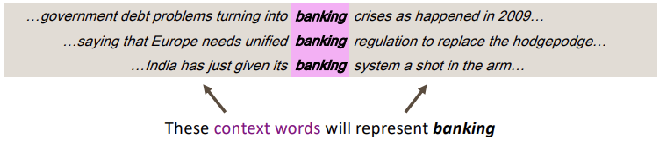
$\mathbf{Fig\ 1.}$ Different meanings of banking (source: Christopher Manning, Stanford CS224n)

Accepting this principle, word2vec selects a vector for each word such that its neighbors are “close” under this representation. In word2vec, we denotes the word that we are interested in, or should predict its meaning as a center word $c$ and other remaining words as context words $o$. For example in $\mathbf{Fig\ 1.}$, "banking" is a center word.

It is possible to create a vector from the words in two different point of view. As we discuss, since the context words determine the meaning of center word, we can construct a representation of center word from other context words. On the other hand, according to the meaning of center word, the representations of context words can be constructed to be close with the center word value. These approaches for constructing a word representation correspond to two different versions of architectures of word2vec: CBoW, and Skip-gram respectively.

Skip-Gram

Then how can we predict the neighbors of a center word from its embedding value? Let’s denote the word in a sentence at position $t$ as $w_t$. Our problem is that for each position $t = 1, \dots, T$, predict context words within a window of fixed size $m$, given center word $w_j$.

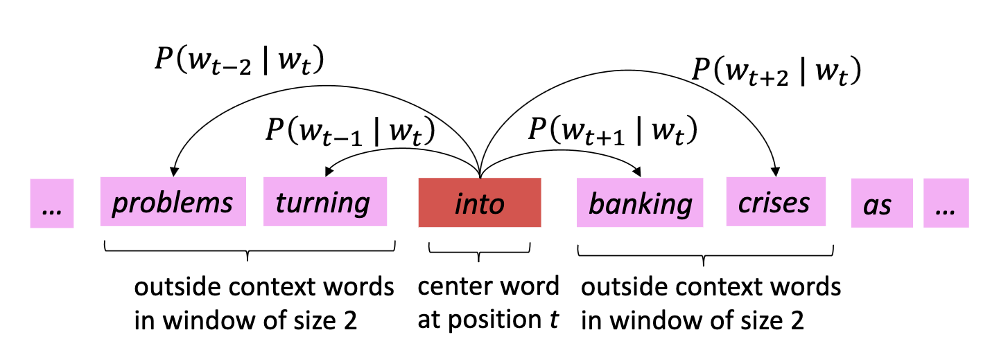
$\mathbf{Fig\ 2.}$ Skip-gram approach (source: Christopher Manning, Stanford CS224n)

We formulate this problem as a maximum likelihood estimation. Note that maximizing the likelihood $L(\theta)$:

\[\begin{aligned} L(\theta) = \prod_{t=1}^T \prod_{\begin{aligned} -m &\leq j \leq m \\ &j \neq 0 \end{aligned}} p(w_{t+j} \mid w_t ; \theta) \end{aligned}\]

is equivalent to minimizing the NLL loss $J(\theta)$:

\[\begin{aligned} J(\theta) = - \frac{1}{T} \text{ log } L(\theta) = - \frac{1}{T} \sum_{t=1}^T \sum_{\begin{aligned} -m &\leq j \leq m \\ &j \neq 0 \end{aligned}} \text{ log } p(w_{t+j} \mid w_t ; \theta) \end{aligned}\]

Next problem is to model $p(w_{t+j} \mid w_t ; \theta)$. In word2vec, $p(w_{t+j} \mid w_t ; \theta)$ is modeled by softmax, but employs two vectors per word $w$: $\mathbf{v}_w$ when $w$ is a center word, otherwise $\mathbf{u}_w$. Then, for a center word $c$,context words $o$, and vocabulary $V$,

\[\begin{aligned} p(o \mid c) = \frac{\text{exp}(\mathbf{u}_o^\top \mathbf{v}_c)}{\sum_{w \in V} \text{exp}(\mathbf{u}_w^\top \mathbf{v}_c)} \end{aligned}\]

And by setting the parameter $\theta$ as a vector of these $\mathbf{u}$ and $\mathbf{v}$, the optimal vectors of each word is obtained by

\[\begin{aligned} \underset{\mathbf{u}_1, \dots, \mathbf{u}_n, \mathbf{v}_1, \dots, \mathbf{v}_n}{\text{arg max }} \sum_{c, o} \text{ log } p(o \mid c) \end{aligned}\]

Note that each vector representation can be learned by neural network:

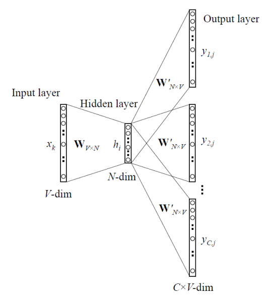
$\mathbf{Fig\ 3.}$ Skip-gram with Neural Network

CBoW

Instead of predicting context words based on the center word, continuous bag of words (CBoW) model predicts the center word from the context. The reason why this architecture is referred to as CBoW is the order of words in the history does not influence the projection and it represents each word by a continuous embedding.

Let $\mathbf{v}_w$ be a vector for the word $w$. And $\bar{\mathbf{v}}_t$ be the average of the word vectors in the window around word $w_t$. If $m$ is the context size,

\[\begin{aligned} \bar{\mathbf{v}}_t = \frac{1}{2m} \sum_{h=1}^m (\mathbf{v}_{w_{t + h}} + \mathbf{v}_{w_{t - h}}) \end{aligned}\]

Let $w_t$ be a center word. Then we formulate \(p(c \mid o) = p (w_t \mid \mathbf{w}_{t-m: t+m})\) as

\[\begin{aligned} p (w_t \mid \mathbf{w}_{t-m: t+m}) = \frac{\text{exp}(\mathbf{v}_{w_t}^\top \bar{\mathbf{v}}_t)}{\sum_{w^\prime \in V} \text{exp}(\mathbf{v}_{w^\prime}^\top \bar{\mathbf{v}}_t)} \end{aligned}\]

The following illustration compares the CBoW and skip-gram models:

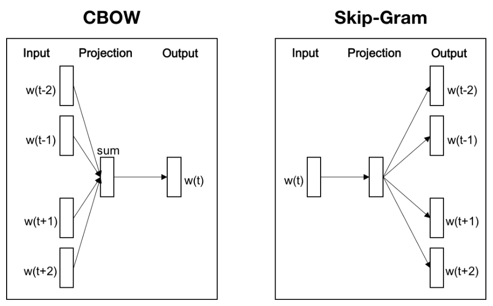
$\mathbf{Fig\ 4.}$ Skip-gram approach (source: Mikolov et al. 2013)

CBoW v.s. Skip-Gram

Intuitively, the task of CBoW (predicting one word from many inputs) is much simpler, this implies a much faster convergence for CBOW than for Skip-gram, in the original paper Mikolov et al. 2013 the authors revealed that CBoW took a day to train, while 3 days for skip-gram model.

And this task difficuly it leads to the ability to learn syntactic and semantic relationships. CBoW captured syntactic relationships between words well while Skip-gram is better in learning better semantic relationships (which is much complex relationship).

Here are some examples of semantic and syntactic questions in the test set they used:

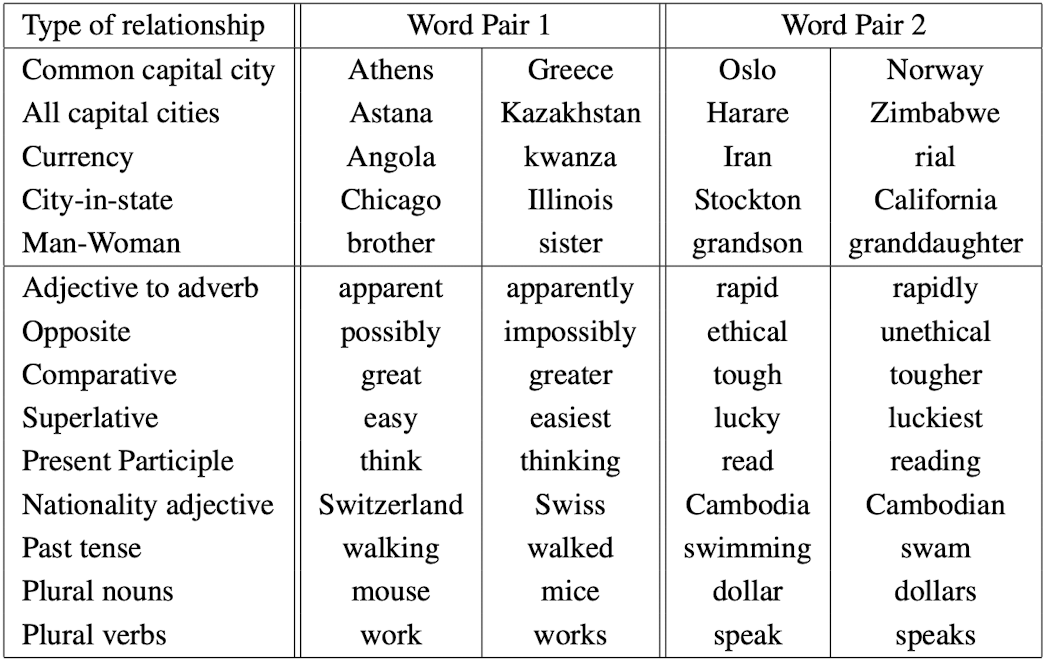
$\mathbf{Fig\ 5.}$ Examples of 5 types of semantic and 9 types of syntactic questions (source: Mikolov et al. 2013)

Finally, in terms of the sensitivity to rare and frequent words, since Skip-gram takes a single center word as an input, it less tends to overfit frequent words. Why? Even if frequent words are presented more times, they still appear individually to the model, while CBoW is prone to overfit because they may be contained several time in the same window of context vectors.

This leads Skip-gram to be also more efficient in term of documents required to achieve good performances, much less than CBOW (and it’s also the reason of the better performances of Skip-gram in capturing semantical relationships).

Negative sampling

Computing the conditional probability of each word using softmax is expensive, due to the denominator that normalizes over all available words in the vocabulary $V$. It significantly slows down the computation of log likelihood and gradient, for both the CBoW and skip-gram models.

Another idea to mitigate inefficiency is to instead set the denominator up as a binary classification. Consider a center word $c$ and a context vector $o$. Denote a label $D = 1$ as an event that the pair $c$ and $o$ actually occurs in the data. And we model

\[\begin{aligned} & P(D = 1 \mid o, c) = \sigma(\mathbf{u}_{o}^\top \mathbf{v}_{c}) = \frac{1}{1 + \text{exp}(-u_o^\top v_c)} \\ & P(D = 0 \mid o, c) = 1 - \sigma(\mathbf{u}_{o}^\top \mathbf{v}_{c}) = \sigma(-\mathbf{u}_{o}^\top \mathbf{v}_{c}) \end{aligned}\]

And, instead of considering all negative words like in the denominator of original $p (o \mid c)$, we train binary logistic regressions for a true pair (center word $c$ and a word in its context window $o$) versus sampled $K$ negative words that do not appear in the current window. To train such a model, the authors set the objective function $J(\theta)$ as

\[\begin{aligned} J_t (\theta) = \text{log } p(D = 1 \mid o, c) + \sum_{k=1}^K p(D = 0 \mid w_k, c) \quad \text{ where } \quad w_k \sim p(w) \end{aligned}\]

for $J(\theta) = \frac{1}{T} \sum_{t=1}^T J_t (\theta)$. Here, the authors employed an unigram distribution for $p(w)$, $p(w) = \frac{\text{freq}(w)^{3/4}}{\sum_{w^\prime \in V} \text{freq}(w^\prime)^{3/4}}$.

Hence, through this objective we can push $v_c$ toward $u_o$, and away from other vectors $u_w$ where $w$ are sampled negative words simultaneously. And this approximated version of skip-gram is also referred to as Skip-gram with negative sampling (SGNS).

Reference

[1] Mikolov, Tomas, et al. “Efficient estimation of word representations in vector space.” arXiv preprint arXiv:1301.3781 (2013).
[2] T. Mikolov, I. Sutskever, K. Chen, G. Corrado, and J. Dean. “Distributed Representa- tions of Words and Phrases and their Compo- sitionality”. In: NIPS. 2013
[3] Stanford CS224n, Natural Language Processing with Deep Learning
[4] UC Berkeley CS182: Deep Learning, Lecture 13 by Sergey Levine
[5] Kevin P. Murphy, Probabilistic Machine Learning: An introduction, MIT Press 2022.
[6] AI StackExchange, What are the main differences between skip-gram and continuous bag of words?