[NLP] ELMo

Word embeddings such as word2vec associate a much better vector representation than just a one-hot vector with each word. However, the vector is consistent even if the word is used in different semantic or syntax. For instance, two sentences "Let's play baseball" and "I saw a play yesterday" involve a word "play" in completely different ways, but the word will have same word2vec representation.

Peters et al. 2018 introduced a new type of word representation called Embeddings from Language Models (ELMo), a deep contextualized word embedding that the representation depends on context. It just sees the entire sentence and assign an embedding for each word via bi-directional language model that is trained on a large corpus of unlabeled text data.

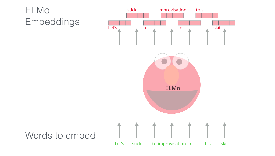
ELMo word embedding (source: Jay Alammar)

---

Bidirectional language models

Consider a multi-layer LSTM model that predict the next word given the word so far in the sentence, which information of previous words is abstracted into a hidden state. But this hidden state is not said to contain the whole context of sentence.

Instead, ELMo word representations are functions of the entire input sentence that are computed on top of multi-layer biLMs. Let a sequnce of $N$ tokens $(x_1, x_2, \dots, x_N)$ be given. The bidirectional Language Model (biLM) associates forward pass and backward pass in a single process.

In the forward pass, model computes the probability of the sequence by modeling the probability of token $x_k$ given the history context:

\[\begin{aligned} p(x_1, \dots, x_n) = \prod_{i=1}^n p(x_i \mid x_1, \dots, x_{i-1}) \end{aligned}\]

In the backward pass, model computes the probability of the sequence by modeling the probability of token $x_k$ given the future context:

\[\begin{aligned} p(x_1, \dots, x_n) = \prod_{i=1}^n p(x_i \mid x_{i + 1}, \dots, x_{n}) \end{aligned}\]

A biLM combines both a forward and backward LM, and the predictions of both directions with hidden states of multi-layer biLSTM \(\overrightarrow{\mathbf{h}}_{i,\ell}\) and \(\overleftarrow{\mathbf{h}}_{i,\ell}\) for input token $x_i$ at $\ell$-th layer and $\ell = 1, \dots, L$. Then the model outputs the probabilities of the next token, by taking a softmax layer.

If we denote the parameter of embedding layer, biLSTM, and softmax layer as $\Theta_e$, \(\overrightarrow{\Theta}_\text{LSTM}\), \(\overleftarrow{\Theta}_\text{LSTM}\) and $\Theta_s$, then the model is trained to jointly maximizes the log likelihood of both directions in unsupervised way:

\[\begin{aligned} \mathcal{L}(\boldsymbol{\Theta}) = \sum_{i=1}^n \Big( \log p(x_i \mid x_1, \dots, x_{i-1}; \Theta_e, \overrightarrow{\Theta}_\text{LSTM}, \Theta_s) + \\ \log p(x_i \mid x_{i+1}, \dots, x_n; \Theta_e, \overleftarrow{\Theta}_\text{LSTM}, \Theta_s) \Big) \end{aligned}\]

The entire architecture of the multi-layer biLSTM model is illustrated in the following figure:

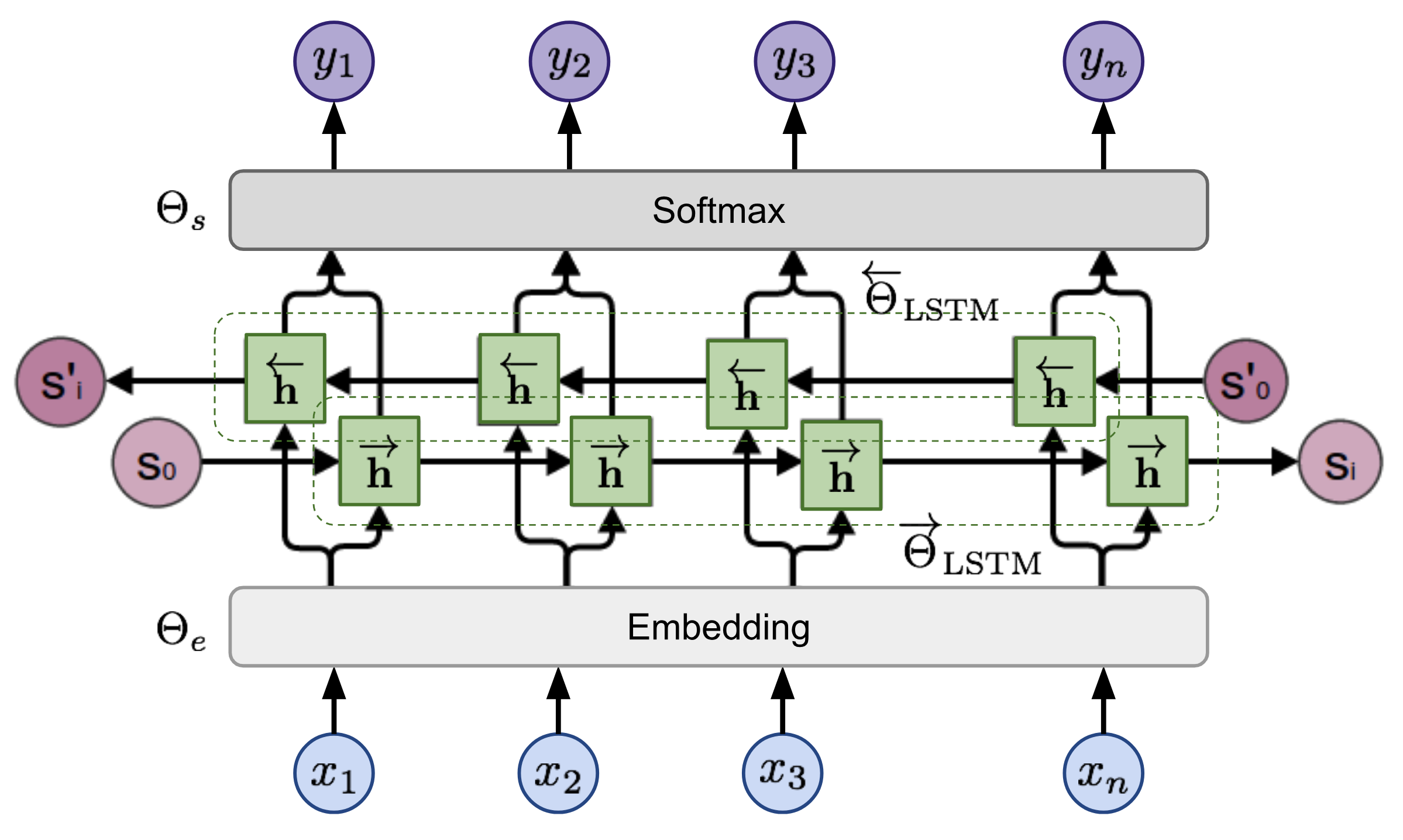
$\mathbf{Fig\ 1.}$ The biLSTM base model of ELMo. (source: Lilian Weng)

ELMo: Embeddings from Language Models

For each token $x_k$, ELMo collects all of its related hidden representations of biLM:

\[\begin{aligned} R_k & = \{ \mathbf{x}_k^{\text{LM}}, \overrightarrow{\mathbf{h}}_{k, \ell}^{\text{LM}}, \overleftarrow{\mathbf{h}}_{k, \ell}^{\text{LM}} \mid \ell = 1, \dots, L \} \\ & = \{ \mathbf{h}_{k, \ell} \mid \ell = 0, \dots, L \} \end{aligned}\]

where \(\mathbf{h}_{k, 0}^{\text{LM}}\) is the output of embedding layer for input token $x_k$ and \(\mathbf{h}_{k, \ell}^{\text{LM}} = [\overrightarrow{\mathbf{h}}_{k,\ell}^{\text{LM}}; \overleftarrow{\mathbf{h}}_{k,\ell}^{\text{LM}}]\).

and collapses all layers into a single vector by function $f(R_k)$ for downstream task. Instead of using a last layer hidden state as an embedding vector, ELMo computes a task specific linear combination of all biLM layers:

\[\begin{aligned} v_k = f(R_k; \Theta^{\text{task}}) = \gamma^{\text{task}} \sum_{\ell = 0}^L s_{\ell}^{\text{task}} \mathbf{h}_{k, \ell}^{\text{LM}}. \end{aligned}\]

where \(\mathbf{s}^{\text{task}}\) are softmax-normalized weights, and the rescale parameter \(\gamma^{\text{task}}\) that compensates the discrepancy between the hidden state distribution and the task specific representations. Note that both parameters are learned for each downstream task i.e., task-specific parameters.

Reference

[1] Peters et al., Deep Contextualized Word Representations, NAACL 2018
[2] UC Berkeley CS182: Deep Learning, Lecture 13 by Sergey Levine
[3] Kevin P. Murphy, Probabilistic Machine Learning: An introduction, MIT Press 2022.