
[NLP] LoRA
Introduction
Many applications in NLP rely on adapting one large language model (LLM) to multiple downstream applications via fine-tuning, which updates all the parameters of the pre-trained model. The major downside of fine-tuning is that the new model contains as many parameters as in the original model. It is seriously inefficient, as LLMs in recent days, such as GPTs, can have billions of parameters.
Hu et al. ICLR 2022 provides an efficient and model-agnostic way for fine-tuning large pre-trained model, termed Low-Rank Adaptation (LoRA). The main idea and hypothesis of LoRA are the observation of intrinsic dimensionality.
The trained over-parameterized models reside on a low intrinsic dimension, and the change in weights during model adaptation also has a low intrinsic rank.
(Although the original paper focused on Transformer language models, the principles of LoRA are still possible to be applied to any dense layers in deep learning models.)
Low-Rank Decomposition of Weight Update $\Delta W$
Let $W_0 \in \mathbb{R}^{d \times k}$ be a pre-trained weight matrix, and $\Delta W$ be a weight update. Based on the hypothesis, LoRA aims to approximate $\Delta W$ with low-rank matrices by decomposing $\Delta W$ into $\Delta W = BA$ where $B \in \mathbb{R}^{d \times r}$ and $A \in \mathbb{R}^{r \times k}$ with the rank $r \ll \min (d, k)$. During training, $W_0$ is frozen and does not receive any gradient signals, while $A$ and $B$ are trainable. (Practically, $A$ is initialized by Gaussian and $B$ is initialized by zero.)
Consequently, the updated forward pass is
\[\begin{aligned} h = (W_0 + \Delta W) \mathbf{x} = W_0 \mathbf{x} + BA \mathbf{x} \end{aligned}\]
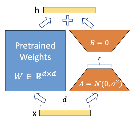
Therefore, LoRA significantly reduces the number of fine-tuning parameters, $dk$ into $dr + rk$. And we can view LoRA as the generalized form of typical fine-tuning. If the rank $r$ of LoRA converges to the rank of $W_0$, the expressiveness of full fine-tuning will be recovered.
![]()
Experiments
In the Transformer architecture, recall that there are 4 weight matrices in the self-attention module $(W_q, W_k, W_v, W_o)$ and two in the MLP module. For the experiment, the authors set \(W_q, W_k, W_v \in \mathbb{R}^{d_{\text{model}} \times d_{\text{model}}}\) and limit to only adapt the attention weights for downstream tasks, freezing the MLP modules.
Performance
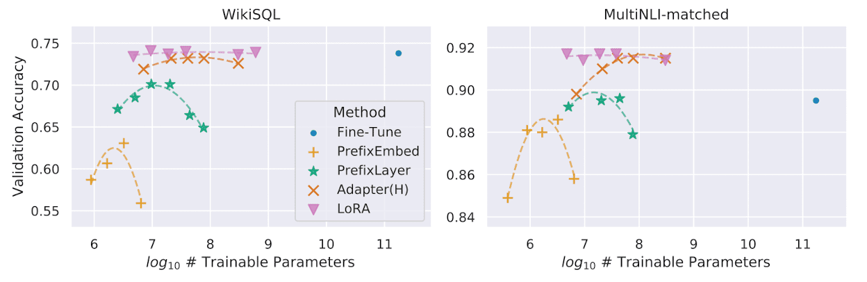
The authors evaluate the downstream task performance of LoRA on various LLMs including RoBERTa, DeBERTa, GPT-2 and GPT-3. And LoRA successfully matches or exceeds the full fine-tuning baselines in most of cases. For example, the next figure shows the validation accuracy v.s. number of trainable parameters of several adaptation methods on GPT-3 with 175B parameters. One can observe that LoRA exhibits better scalability and task performance than other adaptation methods and full fine-tuning.
Optimal $r$
Surprisingly, LoRA performs competitively with a very small $r$, which supports that $\Delta W$ could have a very small intrinsic rank.
![]()
Also, the paper evaluates the overlap of the subspaces learned by different rank $r$ and random seeds, based on the Grassmann distance.
\[\begin{equation} \phi (A_1, A_2, i, j) = \frac{\| U_{A_1}^{i \top} U_{A_2}^j \|_F^2 }{\min (i, j)} \in [0, 1] \end{equation}\]Formal explanation of Grassmann distance
(Reference: Kristian Eschenburg)
Intuitively, we can measure the overlap of subspaces by using the angles between subspaces that tell us how far apart the two subspaces are. Simply, consider the following 2D linear subspaces intersection.
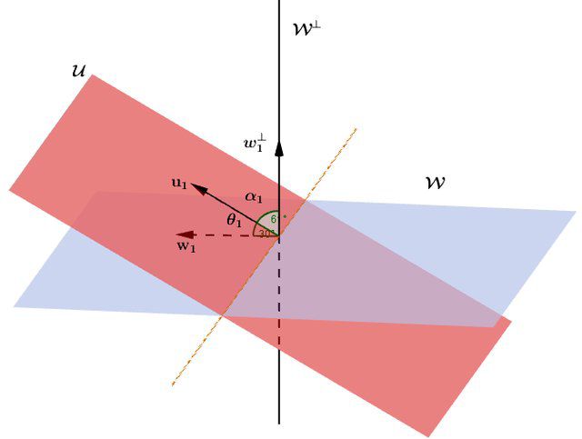
Let any two $r$-dimensional subspaces $U$ and $V$ in $\mathbb{R}^n$ be given. We compute the QR decomposition of $U = Q_u R_u$ and $V = Q_v R_v$ where the columns of $Q_u, Q_v \in \mathbb{R}^{n \times r}$ form orthonormal bases that span $U$ and $V$, respectively. Then, compute inner products matrix $D = Q_u^\top Q_w \in \mathbb{R}^{r \times r}$ and compute the singular value decomposition $D = U \Sigma V^\top$.
Hence, the singular vectors will represent the principal principal angles between $U$ and $V$. In particular, the principal angle is given by $\cos \theta = \sigma_1$, the largest singular value. With these principal angles, One of the most intuitive and simplest way to compute the overlap between two subspaces is $L_2$ norm:
\[\begin{aligned} \psi (U, V) = \sqrt{\sum_{i=1}^r \cos^{-1} (\sigma_i)^2} \end{aligned}\]and this metric is called the Grassmann Distance. Similar to Grassmann distance, in the paper, the authors use the measure of subspace similarity of $A$ and $B$ by the subspace similarity between their column orthonormal matrices $U_A^i \in \mathbb{R}^{d \times i}$ and $U_B^j \in \mathbb{R}^{d \times j}$, obtained by taking top $i$ and $j$ number of columns of the left singular matrices of $A$ and $B$. (Note that columns of left singular matrix in SVD for the orthonormal base of the column space original matrix.)
If we denote the singular values of \({U_A^i}^\top U_B^j\) to be $\sigma_1, \cdots, \sigma_p$ where $p = \min (i, j)$, the measure is defined as
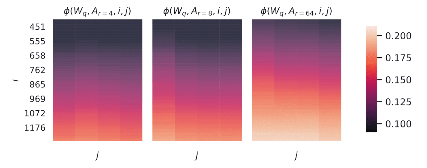
\[\begin{aligned} \phi (A, B, i, j) = \psi (U_A^i, U_B^j) = \frac{\lVert {U_A^i}^\top U_B^j \rVert_F^2}{\min (i, j)} = \frac{\sum_{i = 1}^p \sigma_i^2}{p} \end{aligned}\] \[\tag*{$\blacksquare$}\]$\mathbf{Fig\ 5.}$ shows how \(\phi (A_{r = 8}, A_{r = 64}, i, j)\) ($1 \leq i \leq 8$, $1 \leq j \leq 64$) changes as we vary $i$ and $j$ for given $A_{r = 8}$ and $A_{r = 64}$ which are the learned adaptation matrices with rank $r = 8$ and $64$ using the same pre-trained model. It explains why $r = 1$ performs competitively in downstream tasks for GPT-3:
Directions of the top singular vector overlap significantly, while others do not. Specifically, $\Delta W_v$ (resp. $\Delta W_q$ ) of $A_{r=8}$ and $\Delta W_v$ (resp. $\Delta W_q$) of $A_{r=64}$ share a subspace of dimension 1 with similarity > 0.5.
![]()
In summary, the experiment suggests that increasing $r$ does not cover a more meaningful subspace, which suggests that a low-rank adaptation matrix is sufficient.
Connection between $W$ and $\Delta W$
To evaluate the effect of LoRA, the paper investigate the correlation between $\Delta W$ and $W$, by evaluating whether $\Delta W$ is mostly contained in the top singular directions of $W$ or not.
First, project $W$ onto the $r$-dimensional subspace of $\Delta W$ by computing $U^\top W V^\top$ where $U$ and $V$ are the left and right singular vector matrix of $\Delta W$. Then, compute $\lVert U^\top W V^\top \rVert_F$ and $\lVert W \rVert_F$. As a comparison, we replace $U, V$ with the top $r$ singular vectors of $W$ or a random matrix.
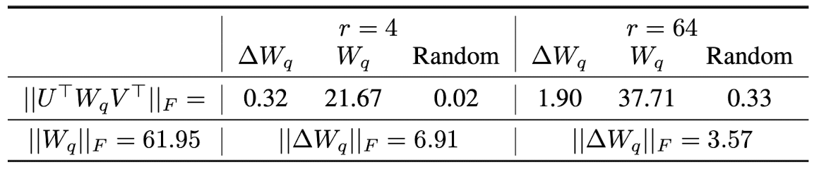
In conclusion,
- $\Delta W$ is highly correlated with $W$ than a random matrix. It suggests that $\Delta W$ amplifies some features already in $W$.
- $\Delta W$ only amplifies directions that are not emphasized in $W$, not repeating the top singular directions of $W$
- the feature amplification factor \(\lVert \Delta W \rVert_F / \lVert U^\top W V^\top \rVert_F\), where $U, V$ are the left/right singular matrices of $\Delta W$, is rather huge when $r$ is small. It provides evidence that the intrinsic rank needed to represent the task-specific directions is low.
In essence, LoRA has the potential to magnify crucial features for particular downstream tasks that were learned but not highlighted (i.e. the low singular vectors) in the general pre-training model.
Reference
[1] Hu et al. “LoRA: Low-Rank Adaptation of Large Language Models” ICLR 2022
[2] Kristian Eschenburg, “Distances Between Subspaces”
Leave a comment