
[RL] Value Function Approximation
Introduction
Most reinforcement learning algorithms covered thus far have utilized tabular storage and updating methods for value functions. In the case of state-value, every state $s$ occupies an entry for $V(s)$, and furthermore, every combinations of states and actions $(s, a)$ has an entry for storing $Q(s, a)$. However, such approach can be inefficient in terms of memory and time complexity when dealing with large state and action spaces, such as the game Go.
Then, how can we scale up the previous methods for large problems? One possible way is, estimate value function with function approximation theories by regarding $v$ and $q$ as functions $\mathcal{S} \to \mathbb{R}$ and $\mathcal{S} \times \mathcal{A} \to \mathbb{R}$.
\[\begin{aligned} & \widehat{v} (S, \mathbf{w}) \approx v_\pi (s) \\ & \widehat{q} (S, A, \mathbf{w}) \approx q_\pi (s, a) \end{aligned}\]by adjusting the parameter $\mathbf{w}$ with gradient descent like a regression. Our goal is to minimize mean-squared error between approximation value function $\widehat{v}(s, \mathbf{w})$ and true value function $v_\pi (s)$. For simplicity, assume that true value function $v_\pi$ is given.
\[\begin{aligned} L (\mathbf{w}) & = \mathbb{E}_\pi \left[ \left(v_\pi (S) - \widehat{v}(S, \mathbf{w}) \right)^2 \right] \\ \nabla_{\mathbf{w}} L (\mathbf{w}) & \propto \mathbb{E}_\pi \left[ (v_\pi (S) - \widehat{v} (S, \mathbf{w})) \cdot \nabla_{\mathbf{w}} \widehat{v}(S, \mathbf{w}) \right] \\ \end{aligned}\]Function approximation methods offer a solution for tasks with arbitrarily large state spaces, where conventional state or state-action tables are impractical due to memory constraints or an inability to optimally fill them even with infinite time and data. Take, for instance, an autonomous car camera capturing diverse images—it’s unlikely to capture the exact same image repeatedly, but it will encounter scenarios it can generalize (e.g., “a single pedestrian walking on the zebra crossing”). In such scenarios, the goal is to achieve generalization and find a good approximate solution with limited computational resources, as an optimal solution is unattainable.
While theoretically, all supervised learning methods can be applied to RL tasks, in practice, we often employ linear function approximators or artificial neural networks (ANNs).
Example: Linear Regression
Let’s just think of it as a linear regression problem in machine learning simply. For feature engineering, an observed state can be represented by a feature vector
\[\begin{aligned} \mathbf{x}(S)=\left(\begin{array}{c} \mathbf{x}_1(S) \\ \vdots \\ \mathbf{x}_n(S) \end{array}\right) \end{aligned}\]like distance of robot from landmarks, etc. With feature vector, we can design a linear model \(\mathbf{x}(S)^\top \mathbf{w} = \sum_{j=1}^n \mathbf{x}_j (S) \mathbf{w}_j\) for value function approximator. Then, the objective function turns out that it is quadratic in parameter $\mathbf{w}$, so that SGD converges on global optimum with simple update rule. From \(\nabla_{\mathbf{w}} \widehat{v}(S, \mathbf{w}) = \mathbf{x}(S)\),
\[\begin{aligned} L (\mathbf{w}) & = \mathbb{E}_\pi \left[ \left(v_\pi (S) - \mathbf{x}(S)^\top \mathbf{w} \right)^2 \right] \\ \delta \mathbf{w} & = \alpha \cdot (v_\pi (S) - \widehat{v}(S, \mathbf{w})) \cdot \mathbf{x}(S) \end{aligned}\]However, we do not have an access to true $v_\pi$ in the reality and only reward signal is a supervisor to the agent. In practice, we usually predict $v_\pi$ with
- Sampling $G_t$ (Monte-Carlo Learning)
- Bootstrapping (TD Learning)
Incremental Approach
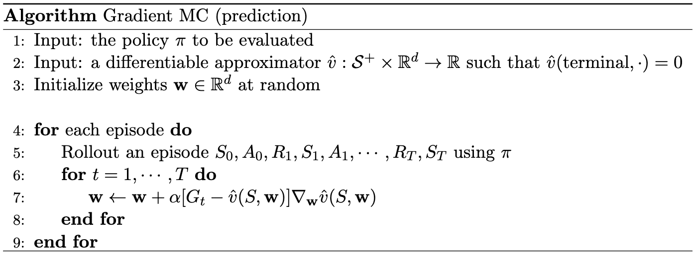
Gradient Monte-Carlo
Note that return $G_t$ is an unbiased (but high variance) random sample of true value $v_\pi (S_t)$. Hence, via Monte Carlo methods, the value function can be trained to output appropriate value when the agent has encountered a state $S$, with training data \(\left\langle S_1, G_1 \right\rangle, \left\langle S_2, G_2 \right\rangle, \cdots, \left\langle S_T, G_T \right\rangle\). Since $G_t$ is an
\[\begin{aligned} \delta \mathbf{w} = \alpha \cdot (G_t - \widehat{v}(S_t, \mathbf{w})) \cdot \nabla_{\mathbf{w}} \widehat{v}(S_t, \mathbf{w}) \end{aligned}\]
Also, it can be employed as policy evaluation for incremental control algorithm, and for model-free method we approximate action-value function $\widehat{q} (S, A, \mathbf{w}) \approx q_\pi (S, A)$ instead of $v_\pi$
\[\begin{aligned} L (\mathbf{w}) & = \mathbb{E}_\pi \left[ \left(q_\pi (S, A) - \widehat{q}(S, A, \mathbf{w}) \right)^2 \right] \\ \nabla_{\mathbf{w}} L (\mathbf{w}) & \propto \mathbb{E}_\pi \left[ (q_\pi (S, A) - \widehat{q} (S, A, \mathbf{w})) \cdot \nabla_{\mathbf{w}} \widehat{q}(S, A, \mathbf{w}) \right] \\ \delta \mathbf{w} & = \alpha \cdot (q_\pi (S, A) - \widehat{q} (S, A, \mathbf{w})) \cdot \nabla_{\mathbf{w}} \widehat{q} (S, A, \mathbf{w}) \end{aligned}\]by replacing $q_\pi (S_t, A_t) \approx G_t$.
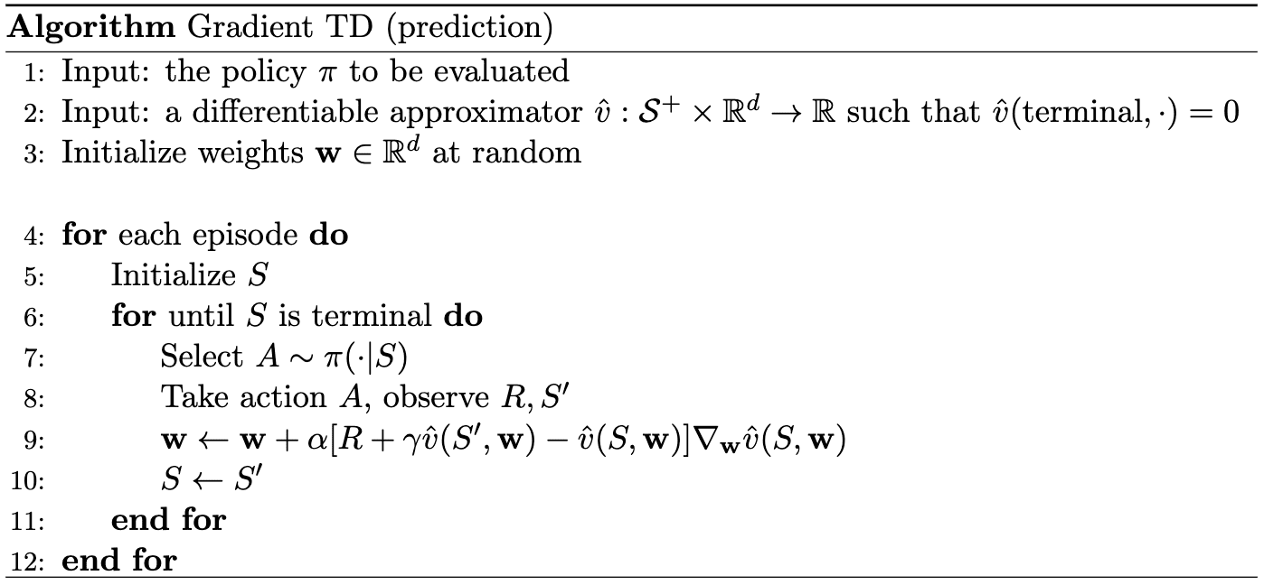
Semi-gradient Temporal Difference (SGTD)
In contrast, TD target $R_{t+1} + \gamma \widehat{v}(S_{t+1}, \mathbf{w})$ is a biased, but much precise sample of true value $v_\pi (S_t)$ due to its bootstrapping nature. For training data \(\left\langle S_1, R_{2} + \gamma \widehat{v}(S_{2}, \mathbf{w}) \right\rangle, \left\langle S_2, R_{3} + \gamma \widehat{v}(S_{3}, \mathbf{w}) \right\rangle, \cdots, \left\langle S_{T-1}, R_T \right\rangle\),
\[\begin{aligned} \delta \mathbf{w} = \alpha \cdot (R_t + \gamma \widehat{v}(S^\prime, \mathbf{w}) - \widehat{v}(S, \mathbf{w})) \cdot \nabla_{\mathbf{w}} \widehat{v}(S, \mathbf{w}) \end{aligned}\]
However, one cannot usually assure the convergence if a bootstrapping estimate is used as the target. Bootstrapping targets such as n-step returns $G_{t: t+ n}$ or TD target indeed depend on the current parameter $\mathbf{w}$, thereby being biased target of true value function $v_\pi$. Moreover, the discussion so far is based on the reasonable belief that the target $v_\pi$ and $q_\pi$ are independent of $\mathbf{w}$. In particular, we assume that
\[\begin{aligned} \nabla_{\mathbf{w}} L (\mathbf{w}) & = \nabla_{\mathbf{w}} \mathbb{E}_\pi \left[ \left(v_\pi (S) - \widehat{v}(S, \mathbf{w})^2 \right)^2 \right] \\ & =\mathbb{E}_\pi \left[ \nabla_{\mathbf{w}} \left(v_\pi (S) - \widehat{v}(S, \mathbf{w})^2 \right)^2 \right] \\ & \propto \mathbb{E}_\pi \left[ \left(v_\pi (S) - \widehat{v}(S, \mathbf{w})\right) \right) \cdot \nabla_{\mathbf{w}} \left(v_\pi (S) - \widehat{v}(S, \mathbf{w}) \right] \\ & = \mathbb{E}_\pi \left[ \left(v_\pi (S) - \widehat{v}(S, \mathbf{w}) \right) \cdot \nabla_{\mathbf{w}} \widehat{v}(S, \mathbf{w}) \right] \\ \end{aligned}\]i.e. $\nabla_{\mathbf{w}} v_\pi (S) = 0$. Hence, our update is not the true gradient descent and includes only a part of the gradient, ignoring the effect of $\mathbf{w}$ on the target. Due to this reason, the algorithm is commonly referred to as semi-gradient methods.
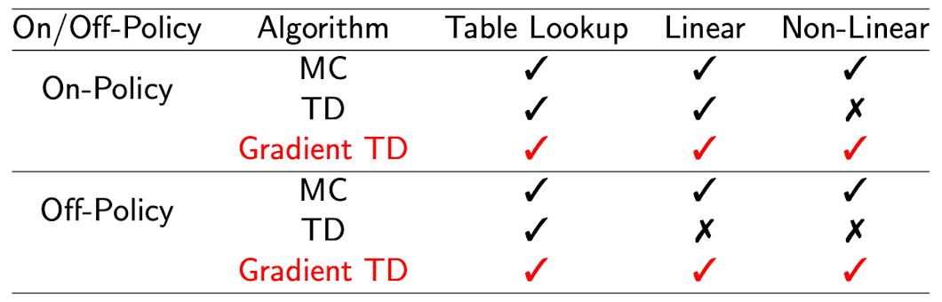
While semi-gradient methods may not offer convergence guarantees as robustly as gradient methods, and even diverges on off-policy setup, they still hold practical merit. Semi-gradient TD methods, for instance, exhibit convergence in certain crucial scenarios, particularly when employing linear function approximation. Moreover, temporal difference learning facilitates rapid, continual, and online training, irrespective of whether the tasks at hand are episodic or continuous in nature. And if we employ the true gradient of projected Bellman error, we call it as a gradient TD and it is known that the convergence is guaranteed even for non-linear approximation. See [2, 4, 5] for more details.
Batch Approach
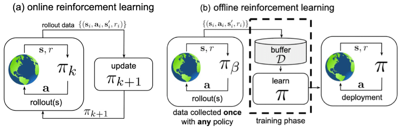
The incremental methods we have discussed perform $n$ sequential updates for each data pair; for instance, in case of gradient MC \(\{ (S_t, G_t) : t = 1, \cdots, T \}\), and discard them after each update. While this may be memory-efficient, it tends to be sample inefficient. In contrast, batch RL aims to determine the optimal value function according to the agent’s experience, which corresponds to training dataset $\mathcal{D}$.
It is important to note that, unlike incremental RL, we do not update our estimation as data arrives. Instead, we store the entire dataset first and initiate the update procedure. As a result, batch RL is commonly referred to as offline RL, while incremental RL is known as online RL.
Least-Squares TD (LSTD)
Batch RL shines a light on its effectiveness, particularly in the realm of linear approximation. This approach allows for the discovery of solutions through direct and straightforward linear algebra operations, obviating the necessity for iterative weight updates until convergence. The incremental algorithms require relatively little computation per time step, but they use information of samples rather inefficiently and requires time steps. The least-square TD (LSTD), a least-squares version of the TD algorithm, leverages a linear function approximator $\widehat{v}(S, \mathbf{w}) = \mathbf{w}^\top \mathbf{x} (S)$ to approximate the true value $v_\pi (S)$. While least-squares algorithms entail more computational effort per time step, they typically demand significantly fewer time steps to attain a specified level of accuracy compared to incremental methods with lower variance.
As we mentioned it earlier, it is proved mathematically that the semi-gradient TD algorithm with linear approximator converges to unique fixed point. To find that fixed point, consider the update of the parameter for each timestep $t$
\[\begin{aligned} \mathbf{w}_{t+1} & = \mathbf{w}_t + \alpha (R_{t+1} + \gamma \mathbf{w}^\top \mathbf{x}_{t+1} - \mathbf{w}_t^\top \mathbf{x}_t) \mathbf{x}_t \\ & = \mathbf{w}_t + \alpha (R_{t+1} \mathbf{x}_t - \mathbf{x}_t (\mathbf{x}_t - \gamma \mathbf{x}_{t+1})^\top \mathbf{w}_t) \end{aligned}\]where \(\mathbf{x}_t = \mathbf{x}(S_t)\). Then, the expected weight parameter of the next timestep can be rewritten as
\[\begin{aligned} \mathbb{E}[\mathbf{w}_{t+1} | \mathbf{w}_t] = \mathbf{w}_t + \alpha (\mathbf{b} - \mathbf{A} \mathbf{w}_t) \end{aligned}\]where \(\mathbf{A} = \mathbb{E} [ \mathbf{x}_t ( \mathbf{x}_t - \gamma \mathbf{x}_{t+1})^\top ] \in \mathbb{R}^{d \times d}\) and \(\mathbf{b} = \mathbb{E}[R_{t+1} \mathbf{x}_t] \in \mathbb{R}^d\). Hence, if the algorithm converges, the parameter should satisfy \(\mathbf{b} = \mathbf{A} \mathbf{w}_{\text{TD}}\), i.e., the update term should be zero. And for positive definite $\mathbf{A}$ we obtain \(\mathbf{w}_{\text{TD}} = \mathbf{A}^{-1} \mathbf{b}\).
However, in practice the true $\mathbf{A}$ and $\mathbf{b}$ are usually unknown, since it is the expected value. To handle this unavailability, we approximate them via MC estimation
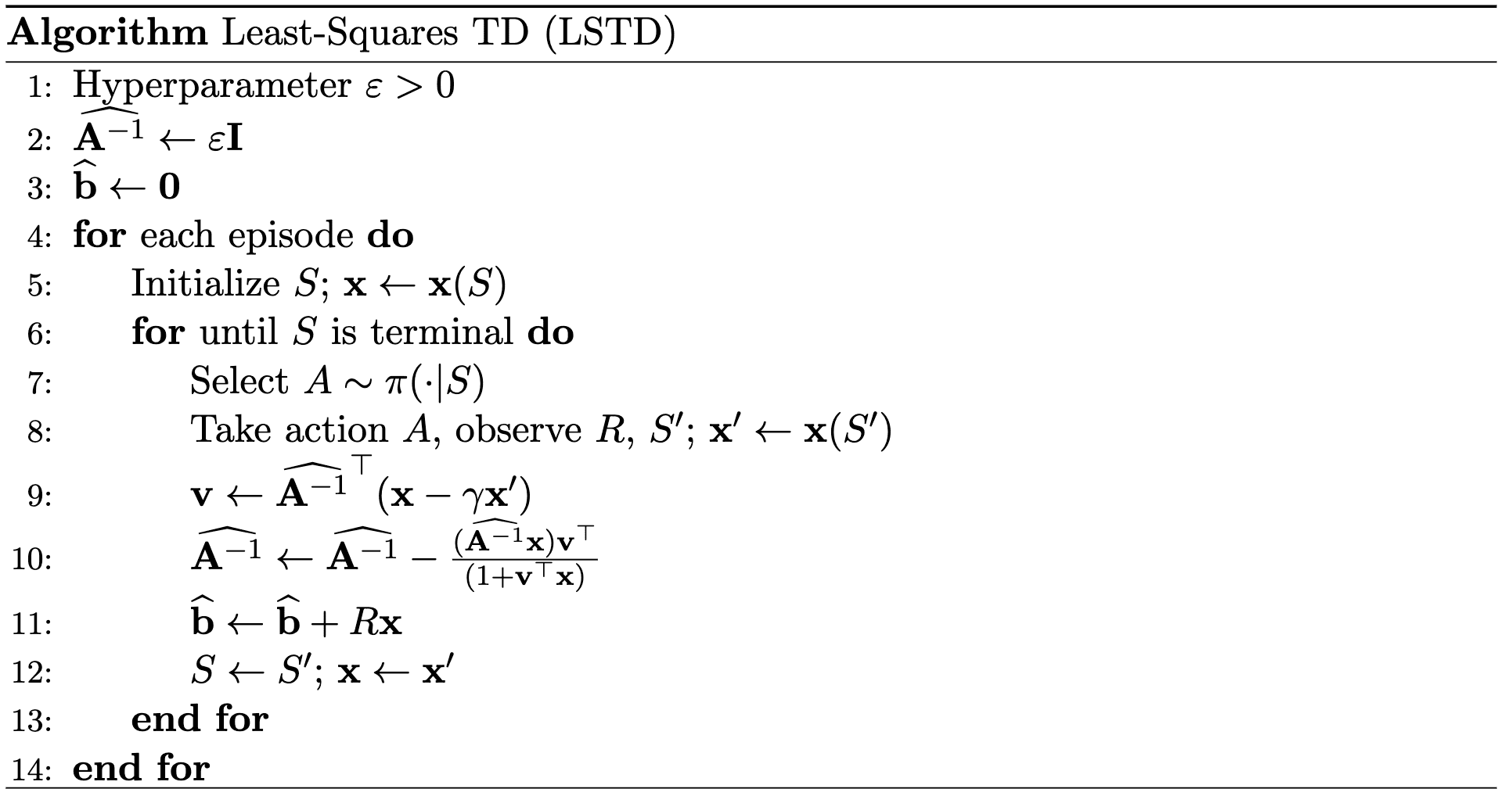
\[\begin{aligned} \widehat{\mathbf{A}}_t & = \sum_{k=0}^{t-1} \mathbf{x}_k (\mathbf{x}_k - \gamma \mathbf{x}_{t+1})^\top + \varepsilon \mathbf{I} \\ \widehat{b}_t & = \sum_{k=0}^{t-1} R_{t+1} \mathbf{x}_k \end{aligned}\]where $\varepsilon \mathbf{I}$ term in order to the invertibility of $\widehat{\mathbf{A}}_t$ every step. The main difference between Least-Squares TD (LSTD) and semi-gradient TD (SGTD) is, LSTD find the optimal solution that is closest to \(\mathbf{w}_{\text{TD}}\) directly with least squares algorithm, whereas SGTD iteratively updates $\mathbf{w}$ toward \(\mathbf{w}_{\text{TD}}\). (Hence, LSTD is an example of batch RL as it requires the complete dataset to the algorithm.)
In practice, to avoid the inverse operation which costs $O(d^3)$, the Sherman-Morrison formula is leveraged to speed up the algorithm to be $O(d^2)$ by incrementally updating:
\[\begin{aligned} \widehat{\mathbf{A}}_t^{-1} & =\left(\widehat{\mathbf{A}}_{t-1}+\mathbf{x}_{t-1}\left(\mathbf{x}_{t-1}-\gamma \mathbf{x}_t\right)^{\top}\right)^{-1} \\ & =\widehat{\mathbf{A}}_{t-1}^{-1}-\frac{\widehat{\mathbf{A}}_{t-1}^{-1} \mathbf{x}_{t-1}\left(\mathbf{x}_{t-1}-\gamma \mathbf{x}_t\right)^{\top} \widehat{\mathbf{A}}_{t-1}^{-1}}{1+\left(\mathbf{x}_{t-1}-\gamma \mathbf{x}_t\right)^{\top} \widehat{\mathbf{A}}_{t-1}^{-1} \mathbf{x}_{t-1}} \end{aligned}\]for $t>0$, with $\widehat{\mathbf{A}} = \varepsilon \mathbf{I}$.
Undoubtedly, the computational expense of $O(d^2)$ associated with LSTD remains significantly higher than the $O(d)$ complexity of semi-gradient TD methods. Therefore, the effectiveness of adopting LSTD depends upon several factors; how large $d$ is, how important it is to learn quickly, and the cost implications of other components within the system.
Deep Q-Learning and Deep Q-Network (DQN)
After approximating the value function \(\widehat{v}_{\mathbf{w}} \approx v_\pi\), now we can obtain the optimal policy $\pi^*$ via policy improvement process with \(\widehat{v}_{\mathbf{w}}\). However, recall that in greedy policy improvement over \(v(\mathbf{s})\), it necessitates the model of MDP to find an improved policy:
\[\pi^\prime (\mathbf{s}) = \underset{\mathbf{a} \in \mathcal{A}}{\text{ argmax }} \left[ \mathcal{r}(\mathbf{s}, \mathbf{a}) + \gamma \sum_{\mathbf{s}^\prime \in \mathcal{S}} \mathcal{P}_{\mathbf{s}\mathbf{s}^\prime}^\mathbf{a} v(\mathbf{s}^\prime) \right]\]It is because we need to take an action at least once and compare an action value \(q(\mathbf{s}, \mathbf{a})\) to know the optimality of action. Hence, once we know $q(\mathbf{s}, \mathbf{a})$ for all action $\mathbf{a} \in \mathcal{A}$, we can improve the policy without MDP model. To eliminate the need for an MDP model, we now consider to estimate an action-value $q_\pi$ instead of $v_\pi$.
Suppose we represent the state-action value function by a deep neural network, $\widehat{q}_{\mathbf{w}} (\mathbf{s}, \mathbf{a})$ called Q-network with weights $\mathbf{w}$. To find the optimal $\mathbf{w}$, we minimize the MSE as usual:
\[\begin{aligned} \mathcal{L}(\mathbf{w}) & = \mathbb{E}_\pi \left[ (q_\pi (\mathbf{s}, \mathbf{a}) - \widehat{q}_\mathbf{w} (\mathbf{s}, \mathbf{a}))^2 \right] \\ \nabla_{\mathbf{w}} \mathcal{L}(\mathbf{w}) & = \mathbb{E}_\pi \left[ \left( q_\pi (\mathbf{s}, \mathbf{a}) - \widehat{q}_\mathbf{w} (\mathbf{s}, \mathbf{a}) \right) \cdot \nabla_{\mathbf{w}} \widehat{q}_\mathbf{w} (\mathbf{s}, \mathbf{a}) \right]. \end{aligned}\]And simultaneously, we need to optimize the $q_\pi (\mathbf{s}, \mathbf{a})$ to obtain the optimal Q-value $Q^* (\mathbf{s}, \mathbf{a})$. Hence, we may approximate the unavailable target $q_\pi (\mathbf{s}, \mathbf{a})$ by $r + \gamma \underset{\mathbf{a}^\prime}{\max} \widehat{q}_{\mathbf{w}} (\mathbf{s}^\prime, \mathbf{a}^\prime)$ as Q-Learning:
\[\nabla_{\mathbf{w}} \mathcal{L}(\mathbf{w}) \approx \mathbb{E}_\pi \left[ \left( r + \gamma \underset{\mathbf{a}^\prime}{\max} \widehat{q}_{\mathbf{w}} (\mathbf{s}^\prime, \mathbf{a}^\prime) - \widehat{q}_\mathbf{w} (\mathbf{s}, \mathbf{a}) \right) \cdot \nabla_{\mathbf{w}} \widehat{q}_\mathbf{w} (\mathbf{s}, \mathbf{a}) \right].\]If the weights are updated after every time-step, and the expectations are replaced by single samples from the behaviour distribution $\rho$ and the transition \(\mathcal{P}_{\mathbf{s}\mathbf{s}^\prime}^\mathbf{a}\) respectively, then this algorithm is equivalent to the Q-learning algorithm, therby being model-free and off-policy; it learns about the greedy strategy $\mathbf{a} = \underset{\mathbf{a}}{\max} \widehat{q}_{\mathbf{w}} (\mathbf{s}^\prime, \mathbf{a}^\prime)$, while following a behaviour distribution $\pi$.
However, again, this approximation faces two main challenges that cause the algorithm diverge:
- strong correlations between consecutive samples, which break the fundamental assumptions (and requirements) of SGD optimization
- non-stationary target, dependent on the parameter of approximator that leads to unstable training
To mitigate the issues, in deep Q-learning, especially deep Q-Networks (DQN) addresses both challenges by experience replay and temporary fixed Q-targets.
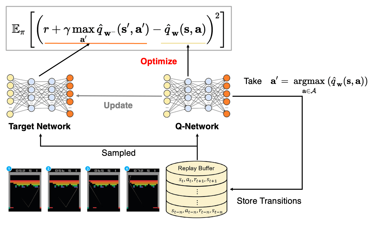
- Experience Replay
To alleviate correlations, we utilize a replay buffer to store datasets from prior experiences. As the agent interact with the environment, tuples are gradually added to the buffer. A straightforward implementation is using a buffer with a fixed size, where new data is appended to the end of the buffer, evicting the oldest experience.
The process of sampling a small batch of tuples from the replay buffer for training the neural network is termed experience replay. Beyond mitigating correlations, it enables us to leverage individual tuples multiple times, thereby enhancing the agent's ability to extract valuable insights from experiences.
During training, we uniformly sample a batch of experience tuples $(\mathbf{s}, \mathbf{a}, r, \mathbf{s}^\prime)$ randomly from the replay buffer, and subsequently compute the loss function with these tuples. - Fixed Q-Targets
To enchance stability, DQN circumvents the non-stationary target by fixing the target weights $\mathbf{w}^-$ for multiple updates. Note that it still serves as an estimate of the true value function.
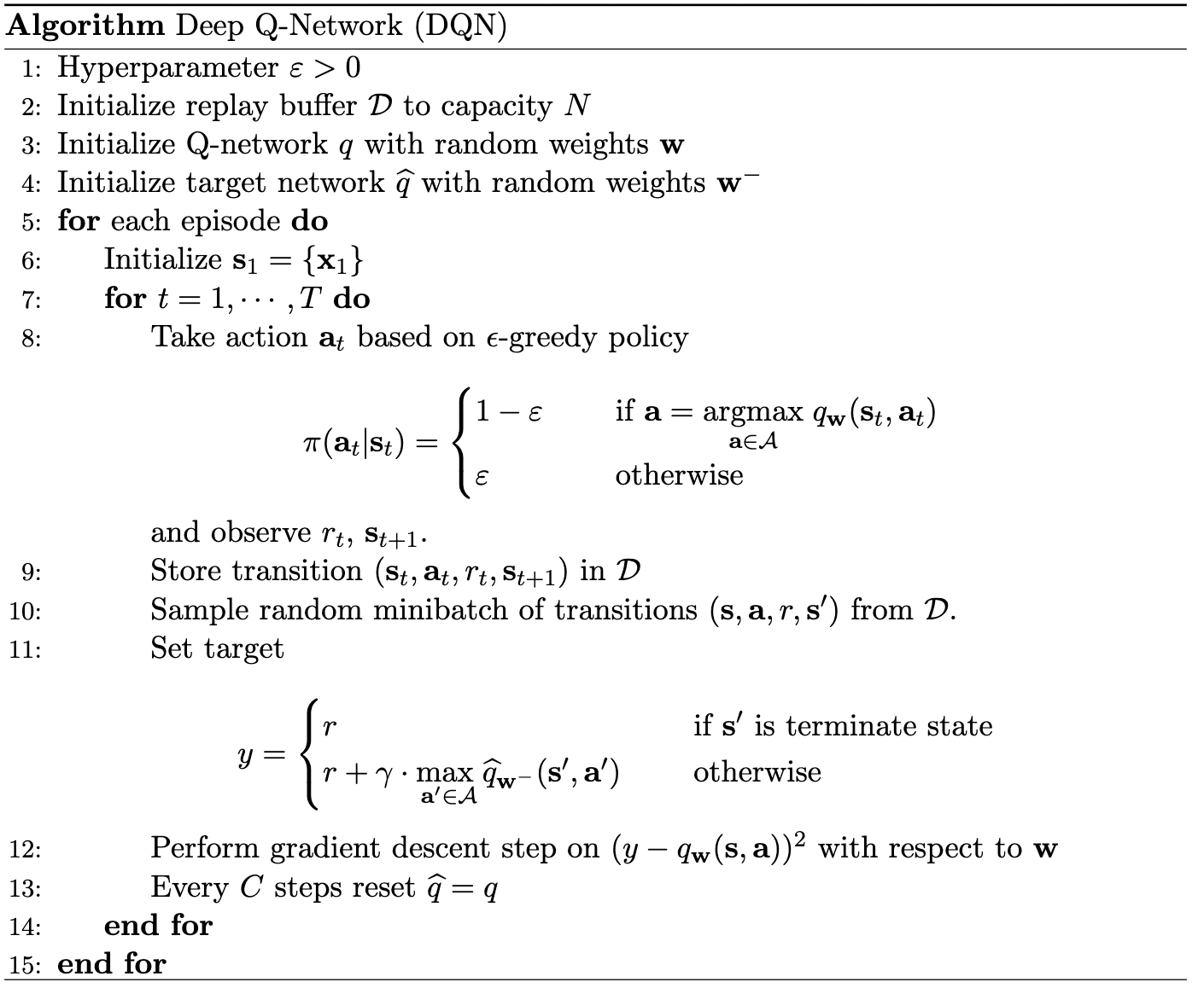
Then, initially, we create a copy of the neural network, denoted as the target network $\widehat{q}_{\mathbf{w}^-} (\mathbf{s}^\prime, \mathbf{a}^\prime)$ to calculate the Q-learning target, from the Q-network $\widehat{q}_\mathbf{w} (\mathbf{s}, \mathbf{a})$. Subsequently, we periodically update the target network by copying the weights from the Q-network, specifically every $C$ training updates. In other words, the weight of Q-network $\mathbf{W}$ are are updated for each tuple sample during the training process, while the weights in the target network are copied less frequently from the Q-network.
The DQN algorithm can be described as the following pseudocode:
Reference
[1] Introduction to Reinforcement Learning with David Silver
[2] A (Long) Peek into Reinforcement Learning
[3] Stanford CS234: Reinforcement Learning
[4] Rao, Ashwin, and Tikhon Jelvis. Foundations of reinforcement learning with applications in finance. Chapman and Hall/CRC, 2022.
[5] Brandfonbrene et al. “Geometric Insights into the Convergence of Nonlinear TD Learning”, ICLR 2020
[6] Bradtke, Steven J., and Andrew G. Barto. “Linear least-squares algorithms for temporal difference learning.” Machine learning 22.1 (1996): 33-57.
[7] Mnih et al. “Playing Atari with Deep Reinforcement Learning”, NIPS Workshop 2013
[8] Mnih et al. “Human-level control through deep reinforcement learning”, Nature 2015
Leave a comment