
[RL] Policy Gradient
So far, we considered some various ways for computing values such as Monte-Carlo estimation, Temporal-Difference learning, and also we approximate them using parameters $\theta$ by $V_\theta (\mathbf{s}) \approx V^\pi (\mathbf{s})$. These kinds of algorithms are called value-based RL, since it learns value functions and generate a policy directly from the learnt value function. Policy was induce by value function for
In this post, we will directly parametrize the policy by
\[\begin{aligned} \pi_\theta (\mathbf{a} \vert \mathbf{s}) = P(\mathbf{a} \vert \mathbf{s}, \theta ) \end{aligned}\]without knowledge of MDP environment. And such a way is known as Policy-based RL. Policy-based RL has better convergence properties and also effective in high-dimensional or continuous action spaces. It also has the advantage of capability of learning stochastic policies. (There are some cases that a stochastic policy is an optimal instead of greedy one.)

Direct Policy Differentiation
Now, our policy is parametrized by $\theta$. And, we want to find \(\theta^*\) that uniformly maximizes the value of all states. Then, to find a policy that is as better as possible across the entire state space, one may set the objective by
\[\begin{aligned} \theta^* & = \underset{\theta}{\text{ argmax }} J(\theta) \\ & = \underset{\theta}{\text{ argmax }} \mathbb{E}_{\mathbf{s}_0} \left[ V^{\pi_\theta} (\mathbf{s}_0) \right] \\ & = \underset{\theta}{\text{ argmax }} \mathbb{E}_{\tau \sim p_\theta (\tau)} \left[ \underset{t = 1}{\sum} \gamma^t r (\mathbf{s}_t, \mathbf{a}_t) \right] \\ & \approx \underset{\theta}{\text{ argmax }} \frac{1}{N} \sum_{i=1}^N \underset{t = 1}{\sum} \gamma^t r (\mathbf{s}_{i, t}, \mathbf{a}_{i, t})) \end{aligned}\]where sampled trajectories follow
\[\begin{aligned} p_\theta (\tau) & = p_\theta (\mathbf{s}_1, \mathbf{a}_1, \cdots, \mathbf{s}_T, \mathbf{a}_T) \\ & = p(\mathbf{s}_1) \prod_{t=1}^T \pi_\theta (\mathbf{a}_t \vert \mathbf{s}_t) \cdot p(\mathbf{s}_{t+1} \vert \mathbf{s}_t, \mathbf{a}_t) \end{aligned}\]But this objective is not easy to compute gradient w.r.t. $\theta$ :
\[\begin{aligned} \nabla_\theta J(\theta) & =\nabla_\theta \mathbb{E}_{\tau \sim p_\theta}[G(\tau)] \\ & =\nabla_\theta \int p_\theta(\tau) G(\tau) d \tau \\ & =\int \nabla_\theta p_\theta(\tau) G(\tau) d \tau \quad \leftarrow \text { Difficult to compute } \end{aligned}\]In $p_\theta$, a model of environment $p(\mathbf{s}_{t+1} \vert \mathbf{s}_t, \mathbf{a}_t)$ is incorporated, so that we cannot compute if MDP model is unknown and even if it is known, like model-based RL, it is sometimes complex. Furthermore, trajectory rollout relies on sampling of the environment, thereby breaking down the computation graph of gradient flow, which makes it impractical to compute in the majority of cases. Hence, it is infeasible to compute in most of the cases. Instead, by log-gradient trick (in some literatures, this gradient is also known as likelihood-ratio gradient):
\[\begin{aligned} \nabla_\theta p_\theta (\tau) = p_\theta (\tau) \frac{\nabla_\theta p_\theta (\tau)}{p_\theta (\tau)} = p_\theta (\tau) \nabla_\theta \text{ log } p_\theta (\tau) \end{aligned}\]it becomes
\[\begin{aligned} \nabla_\theta J(\theta) & =\nabla_\theta \int p_\theta(\tau) G(\tau) d \tau \\ & =\int p_\theta(\tau) \nabla_\theta \text{ log } p_\theta (\tau) G(\tau) d \tau \\ & =\mathbb{E}_{\tau \sim p_\theta} [\nabla_\theta \text{ log } p_\theta (\tau) G(\tau)] \end{aligned}\]where the transition probabilities are removed at all in the gradient by additive property of log function
\[\begin{aligned} \nabla_\theta \text{ log } p_\theta (\tau) & = \sum_{t=1}^T \nabla_\theta \text{ log } \pi_\theta (\mathbf{a}_t \vert \mathbf{s}_t) \end{aligned}\]Now, we can obtain numerical value of gradient
\[\begin{aligned} \nabla_\theta J(\theta) & = \mathbb{E}_{\tau \sim p_\theta} \left[ \left ( \sum_{t=1}^T \nabla_\theta \text{ log } \pi_\theta (\mathbf{a}_{t} \vert \mathbf{s}_{t}) \right ) G(\tau) \right] \\ & \approx \frac{1}{N} \left[ \sum_{i=1}^N \left( \sum_{t=1}^T \nabla_\theta \text{ log } \pi_\theta (\mathbf{a}_{i, t} \vert \mathbf{s}_{i, t}) \right) \left( \sum_{t=1}^T \gamma^t r (\mathbf{s}_{i, t}, \mathbf{a}_{i, t}) \right) \right] \end{aligned}\]by MC approximation.
Monte-Carlo Policy Gradient (REINFORCE)
However, such a natural gradient estimation usually suffers from high variance. The following algorithm (note that this algorithm is on-policy), summarizes the above procedure:
1. Sample $\{ \tau^i \}$ from $\pi_\theta (\mathbf{a}_t \vert \mathbf{s}_t)$
2. Compute the gradient: $$ \begin{aligned} \nabla_\theta J(\theta) & \approx \frac{1}{N} \left[ \sum_{i=1}^N \left( \sum_{t=1}^T \nabla_\theta \text{ log } \pi_\theta (\mathbf{a}_{i, t} \vert \mathbf{s}_{i, t}) \right) \left( \sum_{t=1}^T \gamma^t r (\mathbf{s}_{i, t}, \mathbf{a}_{i, t}) \right) \right] \end{aligned} $$ 3. Update the policy parameter $\theta$ by $$ \begin{aligned} \theta \leftarrow \theta + \alpha \nabla_\theta V(\theta) \end{aligned} $$

Here are some remarks:
One may devise a supervised learning approach by analyzing the trajectory of proficient practitioners (expert). In practice, Tesla, a leader in electronic vehicles, adopted this method for their self-driving technology, and such a way of learning is called imitation learning.


2. Connection with Monte-Carlo estimation
Also, note that it can be seen as approximating $Q_\pi (\mathbf{s}, \mathbf{a})$ by Monte-Carlo estimate $$ \begin{aligned} \nabla_\theta J(\theta) & \approx \frac{1}{N} \left[ \sum_{i=1}^N \left( \sum_{t=1}^T \nabla_\theta \text{ log } \pi_\theta (\mathbf{a}_t \vert \mathbf{s}_t) \right) \left( \sum_{t=1}^T \gamma^t r (\mathbf{s}_{i, t}, \mathbf{a}_{i, t}) \right) \right] \\ & = \frac{1}{N} \left[ \sum_{i=1}^N \left( \sum_{t=1}^T \nabla_\theta \text{ log } \pi_\theta (\mathbf{a}_{i, t} \vert \mathbf{s}_{i, t}) \right) \widehat{Q}^\pi_{i, t} \right] \end{aligned} $$ where $\widehat{Q}^\pi_{i, t}$ is an estimate of expected reward if we take action $\mathbf{a}_{i, t}$ in state $\mathbf{s}_{i, t}$.
For example, let’s consider Gaussian policy for $\pi_\theta$:
For instance, the Gaussian distribution is among the most frequently utilized models for continuous action space. Consider a Gaussian policies with known covariance $\Sigma$ (of course, it can be also parametrized) and a mean is modeled by neural network that inputs $\mathbf{s}_t$: $$ \begin{aligned} \pi_\theta (\mathbf{a}_t \vert \mathbf{s}_t) = \mathcal{N} (f_{\text{NN}} (\mathbf{s}_t) ; \Sigma) \end{aligned} $$ And, with simple matrix calculus, it is clear that $$ \begin{aligned} & \text{log } \pi_\theta (\mathbf{a}_t \vert \mathbf{s}_t) = -\frac{1}{2} \lVert f_{\text{NN}} (\mathbf{s}_t) - \mathbf{a}_t \rVert_\Sigma^2 + C \\ \Rightarrow & \nabla_\theta \text{log } \pi_\theta (\mathbf{a}_t \vert \mathbf{s}_t) = -\frac{1}{2} \Sigma^{-1} (f (\mathbf{s}_t) - \mathbf{a}_t ) \frac{df}{d\theta} \end{aligned} $$
Policy Gradient Theorem
So, we formalized the objective $J(\theta)$ as the expected return when following policy $\pi_\theta$, averaged over all states and actions. And as common in machine learning, we directly derived the gradient of $J(\theta)$ with log-gradient trick.
\[\begin{aligned} \nabla_\theta J(\theta) \approx \frac{1}{N} \left[ \sum_{i=1}^N \left( \sum_{t=1}^T \nabla_\theta \text{ log } \pi_\theta (\mathbf{a}_{i, t} \vert \mathbf{s}_{i, t}) \right) \left( \sum_{t=1}^T \gamma^t r (\mathbf{s}_{i, t}, \mathbf{a}_{i, t}) \right) \right] \end{aligned}\]However, Sutton et al. (1999) demonstrated that the estimation of policy gradient can be accomplished by substituting the return of the sampled trajectory with the Q-value of each state-action pair:
For any differentiable policy $\pi_\theta ( a \vert s )$, the policy gradient is $$ \begin{aligned} \nabla_\theta V(\theta) & = \mathbb{E}_{\tau \sim p_\theta} [ \nabla_\theta \text{ log } \pi_\theta (\mathbf{a} \vert \mathbf{s}) Q_{\pi_\theta} (\mathbf{s}, \mathbf{a})] \\ \end{aligned} $$
$\mathbf{Proof.}$ Brief idea of the proof
For simple analysis, let’s assume all trajectories start from a state $\mathbf{s}_0$. In other words, $J(\theta) = V^\pi (\mathbf{s}_0)$. Previously, it was \(J( \theta ) = \mathbb{E}_{\mathbf{s}_0} [V^{\pi_\theta} (\mathbf{s}_0)]\). Note that this assumption doesn’t affect the validity proof, and theorem can be proved for general case in the same way. See p.419 of [5]
\[\begin{aligned} \nabla_\theta V^\pi (\mathbf{s}) & = \nabla_\theta \left( \sum_{\mathbf{a} \in \mathcal{A}} \pi_\theta ( \mathbf{a} \vert \mathbf{s} ) \cdot Q^\pi (\mathbf{s}, \mathbf{a}) \right) \\ & = \sum_{\mathbf{a} \in \mathcal{A}} \nabla_\theta \pi_\theta ( \mathbf{a} \vert \mathbf{s} ) \cdot Q^\pi (\mathbf{s}, \mathbf{a}) + \pi_\theta ( \mathbf{a} \vert \mathbf{s} ) \nabla_\theta Q^\pi (\mathbf{s}, \mathbf{a}) \\ & = \sum_{\mathbf{a} \in \mathcal{A}} \left( \nabla_\theta \pi_\theta ( \mathbf{a} \vert \mathbf{s} ) \cdot Q^\pi (\mathbf{s}, \mathbf{a}) + \pi_\theta ( \mathbf{a} \vert \mathbf{s} ) \nabla_\theta \sum_{\mathbf{s}^\prime, r} P(\mathbf{s}^\prime, r \vert \mathbf{s}, \mathbf{a}) (r + V^\pi (\mathbf{s}^\prime)) \right) \\ & = \sum_{\mathbf{a} \in \mathcal{A}} \left( \nabla_\theta \pi_\theta ( \mathbf{a} \vert \mathbf{s}) \cdot Q^\pi (\mathbf{s}, \mathbf{a}) + \pi_\theta ( \mathbf{a} \vert \mathbf{s} ) \sum_{\mathbf{s}^\prime, r} P(\mathbf{s}^\prime, r \vert \mathbf{s}, \mathbf{a}) \cdot \nabla_\theta V^\pi (\mathbf{s}^\prime) \right) \\ & = \sum_{\mathbf{a} \in \mathcal{A}} \left( \nabla_\theta \pi_\theta ( \mathbf{a} \vert \mathbf{s}) \cdot Q^\pi (\mathbf{s}, \mathbf{a}) + \pi_\theta ( \mathbf{a} \vert \mathbf{s} ) \sum_{\mathbf{s}^\prime} P(\mathbf{s}^\prime \vert \mathbf{s}, \mathbf{a}) \cdot \nabla_\theta V^\pi (\mathbf{s}^\prime) \right) \\ \end{aligned}\]Thus, we obtained a recursive formula of $\nabla_\theta V^\pi (\mathbf{s})$:
\[\begin{aligned} \nabla_\theta V^\pi (\mathbf{s}) = \sum_{\mathbf{a} \in \mathcal{A}} \left( \nabla_\theta \pi_\theta ( \mathbf{a} \vert \mathbf{s}) \cdot Q^\pi (\mathbf{s}, \mathbf{a}) + \pi_\theta ( \mathbf{a} \vert \mathbf{s} ) \sum_{\mathbf{s}^\prime \in \mathcal{S}} P(\mathbf{s}^\prime \vert \mathbf{s}, \mathbf{a}) \cdot \nabla_\theta V^\pi (\mathbf{s}^\prime) \right) \end{aligned}\]Now, we introduce a new notation for further step. Let $\rho^\pi (\mathbf{s} \to \mathbf{x}, k)$ be the probability of transitioning from state $\mathbf{s}$ to $\mathbf{x}$ in $k$ steps. For example,
- $k = 0$ then $\rho^\pi (\mathbf{s} \to \mathbf{s}, 0) = 1$
- $k = 1$ then $\rho^\pi (\mathbf{s} \to \mathbf{s}^\prime, 1) = \sum_{\mathbf{a} \in \mathcal{A}} \pi_\theta (\mathbf{a} \vert \mathbf{s}) p(\mathbf{s}^\prime \vert \mathbf{s}, \mathbf{a})$
- $\rho^\pi (\mathbf{s} \to \mathbf{x}, k + 1) = \sum_{\mathbf{s}^\prime \in \mathcal{S}} \rho^\pi (\mathbf{s} \to \mathbf{s}^\prime, k)$
And, for abbreviation, let $\phi (\mathbf{s}) = \sum_{\mathbf{a} \in \mathcal{A}} \nabla_\theta \pi_\theta ( \mathbf{a} \vert \mathbf{s} ) Q^\pi (\mathbf{s}, \mathbf{a})$. Then,
\[\begin{aligned} \nabla_\theta V^\pi (\mathbf{s}) & = \sum_{\mathbf{a} \in \mathcal{A}} \left( \nabla_\theta \pi_\theta ( \mathbf{a} \vert \mathbf{s} ) \cdot Q^\pi (\mathbf{s}, \mathbf{a}) + \pi_\theta ( \mathbf{a} \vert \mathbf{s} ) \sum_{\mathbf{s}^\prime \in \mathcal{S}} P(\mathbf{s}^\prime \vert \mathbf{s}, \mathbf{a}) \cdot \nabla_\theta V^\pi (\mathbf{s}^\prime) \right) \\ & = \phi (\mathbf{s}) + \sum_{\mathbf{a} \in \mathcal{A}} \pi_\theta ( \mathbf{a} \vert \mathbf{s} ) \sum_{\mathbf{s}^\prime \in \mathcal{S}} P(\mathbf{s}^\prime \vert \mathbf{s}, \mathbf{a}) \cdot \nabla_\theta V^\pi (\mathbf{s}^\prime) \\ & = \phi (\mathbf{s}) + \sum_{\mathbf{s}^\prime \in \mathcal{S}} \sum_{\mathbf{a} \in \mathcal{A}} \pi_\theta ( \mathbf{a} \vert \mathbf{s} ) \cdot P(\mathbf{s}^\prime \vert \mathbf{s}, \mathbf{a}) \cdot \nabla_\theta V^\pi (\mathbf{s}^\prime) \\ & = \phi (\mathbf{s}) + \sum_{\mathbf{s}^\prime \in \mathcal{S}} \rho^\pi (\mathbf{s} \to \mathbf{s}^\prime, 1) \cdot \nabla_\theta V^\pi (\mathbf{s}^\prime) \\ & = \phi (\mathbf{s}) + \sum_{\mathbf{s}^\prime \in \mathcal{S}} \rho^\pi (\mathbf{s} \to \mathbf{s}^\prime, 1) \cdot \nabla_\theta [\phi(\mathbf{s}^\prime) + \sum_{\mathbf{s}^{\prime \prime} \in \mathcal{S}} \rho^\pi (\mathbf{s}^\prime \to \mathbf{s}^{\prime \prime}, 1) \cdot \nabla_\theta V^\pi (\mathbf{s}^{\prime \prime}) ] \\ & = \phi (\mathbf{s}) + \sum_{\mathbf{s}^\prime \in \mathcal{S}} \rho^\pi (\mathbf{s} \to \mathbf{s}^\prime, 1) \phi(\mathbf{s}^\prime) + \sum_{\mathbf{s}^{\prime \prime} \in \mathcal{S}} \rho^\pi (\mathbf{s}^\prime \to \mathbf{s}^{\prime \prime}, 2) \cdot \nabla_\theta V^\pi (\mathbf{s}^{\prime \prime}) \\ & = \phi (\mathbf{s}) + \sum_{\mathbf{s}^\prime \in \mathcal{S}} \rho^\pi (\mathbf{s} \to \mathbf{s}^\prime, 1) \phi(\mathbf{s}^\prime) + \sum_{\mathbf{s}^{\prime \prime} \in \mathcal{S}} \rho^\pi (\mathbf{s} \to \mathbf{s}^{\prime \prime}, 2) \cdot \nabla_\theta V^\pi (\mathbf{s}^{\prime \prime}) + \sum_{\mathbf{s}^{\prime \prime \prime} \in \mathcal{S}} \rho^\pi (\mathbf{s} \to \mathbf{s}^{\prime \prime \prime}, 3) \cdot \nabla_\theta V^\pi (\mathbf{s}^{\prime \prime \prime}) \\ & = \cdots \\ & = \sum_{\mathbf{x} \in \mathcal{S}} \sum_{k = 0}^\infty \rho^\pi (\mathbf{s} \to \mathbf{x}, k) \phi(\mathbf{x}) \end{aligned}\]Note that $k$ starts from $0$, since $\rho^\pi (\mathbf{s} \to \mathbf{x}, 0) = 1$ if and only if $\mathbf{x} = \mathbf{s}$. And $\sum_{k = 0}^\infty \rho^\pi (\mathbf{s} \to \mathbf{x}, k)$ can be interpreted as a preference that how many times the agent started from $s$ visits $x$ in infinite rollout.
Finally, let $\eta (\mathbf{s}) = \sum_{k=0}^\infty \rho^\pi (\mathbf{s}_0 \to \mathbf{s}, k)$.
\[\begin{aligned} \nabla_\theta J(\theta) & = \nabla_\theta V^{\pi_\theta} (\mathbf{s}_0) \\ & = \sum_{\mathbf{s} \in \mathcal{S}} \sum_{k=0}^\infty \rho^\pi (\mathbf{s}_0 \to s, k) \phi(\mathbf{s}) \\ & = \left( \sum_{\mathbf{s} \in \mathcal{S}} \eta (\mathbf{s}) \right) \sum_{\mathbf{s} \in \mathcal{S}} \frac{\eta(\mathbf{s})}{\sum_{\mathbf{s} \in \mathcal{S}} \eta (\mathbf{s})} \phi (\mathbf{s}) \\ & \propto \sum_{\mathbf{s} \in \mathcal{S}} \frac{\eta(\mathbf{s})}{\sum_{\mathbf{s} \in \mathcal{S}} \eta (\mathbf{s})} \phi (\mathbf{s}) \\ & = \sum_{\mathbf{s} \in \mathcal{S}} d^{\pi_\theta} (\mathbf{s}) \sum_{\mathbf{a} \in \mathcal{A}} \nabla_\theta \pi_\theta (\mathbf{a} \vert \mathbf{s}) Q^\pi (\mathbf{s}, \mathbf{a}) \end{aligned}\]Hence,
\[\begin{aligned} \nabla_\theta J(\theta) & = \nabla_\theta V^{\pi_\theta} (\mathbf{s}_0) \\ & \propto \sum_{\mathbf{s} \in \mathcal{S}} d^{\pi_\theta} (\mathbf{s}) \sum_{\mathbf{a} \in \mathcal{A}} \nabla_\theta \pi_\theta (\mathbf{a} \vert \mathbf{s}) Q^\pi (\mathbf{s}, \mathbf{a}) \\ & = \sum_{\mathbf{s} \in \mathcal{S}} d^{\pi_\theta} (\mathbf{s}) \sum_{\mathbf{a} \in \mathcal{A}} \frac{\nabla_\theta \pi_\theta (\mathbf{a} \vert \mathbf{s})}{\pi_\theta (\mathbf{a} \vert \mathbf{s})} Q^\pi (\mathbf{s}, \mathbf{a}) \\ & = \mathbb{E}_{\pi_\theta} [Q^\pi (\mathbf{s}, \mathbf{a}) \nabla_\theta \text{ ln } \pi_\theta ( \mathbf{a} \vert \mathbf{s})]._\blacksquare \end{aligned}\]Actor-Critic Policy Gradient
As mentioned, REINFORCE algorithm has high variance, which is the main fallacy of Monte-Carlo estimation, the convergence of algorithm sometimes takes long time. And that’s why we introduced additional techniques that are helpful to reduce the variance of algorithm.
Instead, another simple way is not to approximate the Q-value by an unbiased sample return, but to use a function approximation with parameters. Such an algorithm is referred to as Actor-Critic Policy Gradient; a policy $\pi_\theta$ is an actor and $Q_w(\mathbf{s}, \mathbf{a})$ is a critic. The actor updates the policy parameters based on the guidance provided by the critic. And, now since Q-value is available, the result of policy gradient theorem in the previous section can be exploited for the gradient ascent.
And in case of training value function, we may employ supervised regression \(\mathcal{L}(\pi) = \frac{1}{2} \sum_{i=1}^N \lVert Q_w (\mathbf{s}_i, \mathbf{a}_i) - y_i \rVert^2\) where $y_i$ is a target, i.e., true \(Q^\pi (\mathbf{s}_i, \mathbf{a}_i)\). Recall that in value function approximation, since true target is usually unknown in the most of tasks, we estimated it through MC and TD. To reduce the variance, we approximate $y_{i, t}$ by TD target (bootstrapping)
\[\begin{aligned} y_{i, t} \approx r(\mathbf{s}_{i, t}, \mathbf{a}_{i, t}) + \gamma \cdot Q_w (\mathbf{s}_{i, t + 1}, \mathbf{a}_{i, t + 1}) \end{aligned}\]Hence, the critique usually takes the form of a TD error.

The benefits of Actor-Critic over REINFORCE are analogous to the distinction between MC and TD methods:
- MC estimate $G_t$ is one-time used and then discarded, so that it’s wasteful.
- Function approximation however makes the experience be accumulated, so that bootstrapping can be used.
- Although it is unbiased, $G_t$ shows high variance.
- Q-Value function updates accumulatively and does not vary enormously, where variance reduction happens.
Q Actor-Critic
The pseudocode of a simple Actor-Critic algorithm is outlined as below:

After each action is selected by actor, the critic evaluates the value to criticize the decision of actor at state $S$.
\[\begin{aligned} \delta_t = r_{t+1} + \gamma Q_w (S_{t+1}, A_{t+1}) - Q_w (S_t, A_t) \end{aligned}\]If $\delta_t$ is positive, it suggests that the tendency to select $A_t$ should be strengthened for the future, whereas if the TD error is negative, it suggests the tendency should be weakened. For true Q-value function, we should find $\mathbf{w}$ which makes $\delta_t = 0$, i.e., $\lVert \delta_t \rVert^2 = 0$. Note that $\delta_t$ is possible to be negative, we should square it for loss function. Thus, a parameter $\mathbf{w}$ is trained by gradient descent:
\[\begin{aligned} \nabla_\mathbf{w} \frac{1}{2} \lVert \delta_t \rVert^2 &= - \delta_t \cdot \nabla_\mathbf{w} Q_\mathbf{w} (S_t, A_t) \end{aligned}\] \[\begin{aligned} \mathbf{w} &\rightarrow \mathbf{w} - \beta \cdot \nabla_\mathbf{w} \frac{1}{2} \lVert \delta_t \rVert^2 \end{aligned}\]Advantage Actor-Critic (A2C)
Recall that subtracting a baseline is a useful technique for reducing algorithmic variance. This approach can also be applied in the Actor-Critic algorithm to reduce the variance. That means,
\[\begin{aligned} \boldsymbol{\theta} \leftarrow \boldsymbol{\theta} + \alpha \cdot \left( Q_\mathbf{w} (\mathbf{s}_t, \mathbf{a}_t) - b(\mathbf{s}_t) \right) \end{aligned}\]And one good selection of the baseline \(b(\mathbf{s}_t)\) is a mean of $Q_\mathbf{w} (\mathbf{s}, \mathbf{a})$ for centering. From \(V_\pi (\mathbf{s}_t) = \mathbb{E}_{\pi (\mathbf{a}_t \vert \mathbf{s}_t)} [Q_{\pi} (\mathbf{s}_t, \mathbf{a}_t)]\), we have
\[\begin{aligned} \nabla_{\boldsymbol{\theta}} J(\boldsymbol{\theta}) = \mathbb{E}_{\pi_{\boldsymbol{\theta}}} \left[ \nabla_{\boldsymbol{\theta}} \text{ log } \pi_{\boldsymbol{\theta}} (\mathbf{s}_t, \mathbf{a}_t) \cdot \left( Q_\mathbf{w} (\mathbf{s}_t, \mathbf{a}_t) - V_\mathbf{v} (\mathbf{s}_t) \right) \right] \end{aligned}\]Note that $V_\mathbf{v} (\mathbf{s}_t)$ is another neural network. And, the difference between Q function and V function $A^\pi (\mathbf{s}, \mathbf{a}) \equiv Q^\pi (\mathbf{s}, \mathbf{a}) - V^\pi (\mathbf{s})$ is usually referred to as advantage function. It indicates how $\mathbf{a}_t$ is advantageous, i.e., provides more value relative to the average value across actions for a given state $\mathbf{s}$. And the above formulation is termed as Advantage Actor-Critic (A2C), operating as follows:

TD Actor-Critic
However, the previous formulation is complex as it requires to learn and save two critic functions. Also, due to the higher-dimensionality of $Q(\mathbf{s}, \mathbf{a}): \mathcal{S} \times \mathcal{A} \to \mathbb{R}$, it is intricate to be approximated and highly unstable. A simpler way to mitigate this issue is to replace action-value by state-value; use the TD error of the state-value function as an estimate of the advantage function. From one sample MC estimation,
\[\begin{aligned} Q^\pi (\mathbf{s}, \mathbf{a}) \approx r(\mathbf{s}, \mathbf{a}) + \gamma \cdot V^\pi (\mathbf{s}^\prime) \end{aligned}\]Then, $\delta_{\mathbf{v}, t} = r(\mathbf{s}, \mathbf{a}) + \gamma \cdot V^\pi (\mathbf{s}^\prime) - V^\pi (\mathbf{s})$ is an unbiased estimate of the advantage function $A^\pi (\mathbf{s}, \mathbf{a})$:
\[\begin{aligned} \mathbb{E}_\pi [\delta_{\mathbf{v}, t} \vert \mathbf{s}, \mathbf{a}] & = \mathbb{E}_\pi [r(\mathbf{s}, \mathbf{a}) + \gamma \cdot V^\pi (\mathbf{s}^\prime) \vert \mathbf{s}, \mathbf{a}] - V^\pi (\mathbf{s}) \\ & = Q^\pi (\mathbf{s}, \mathbf{a}) - V^\pi (\mathbf{s}) \end{aligned}\]Thus, A2C policy gradient can be written in terms of $\delta_{\mathbf{v}, t}$:
\[\begin{aligned} \nabla_{\boldsymbol{\theta}} J(\boldsymbol{\theta}) = \mathbb{E}_{\pi_{\boldsymbol{\theta}}} [\nabla_{\boldsymbol{\theta}} \text{ log } \pi_{\boldsymbol{\theta}} (\mathbf{s}_t, \mathbf{a}_t) \cdot \delta_{\mathbf{v}, t}] \end{aligned}\]Moreover, it necessitates only one neural network for critic, state-value $V$. This algorithm is called TD Actor-Critic:

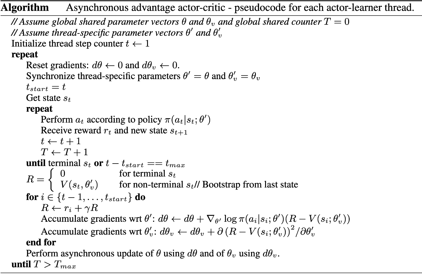
Asynchronous A2C (A3C)
Simple online RL algorithms coupled with deep neural networks face inherent instability due to the non-stationary nature of the sequence of observed data encountered by an online RL agent, as well as the strong correlation among online RL updates. Mitigating this issue involves storing the agent’s data in an experience replay memory, which reduces non-stationarity and decorrelates updates, but at the same time this limits the methods to off-policy RL algorithms.
Alternatively, we can asynchronously execute multiple agents in parallel across multiple instances of the environment. Since at any given time-step the parallel agents experience a variety of different states in this parallelism, it effectively decorrelates the agents’ data, thereby, rendering it more akin to a stationary process. This straightforward yet powerful idea broadens the applicability of a wide spectrum of fundamental on-policy RL algorithms, such as SARSA and n-step methods, as well as off-policy RL algorithms like Q-learning, enabling their robust and effective implementation using deep neural networks without heavy reliance on specialized hardware.
Asynchronous A2C (A3C) is an A2C algorithm adopting this asynchronous parallelism. The critics in A3C learn the value function \(V_{\theta_v} (\mathbf{s}_t)\) while multiple actors \(\pi_{\theta} (\mathbf{a}_t \vert \mathbf{s}_t)\) are trained in parallel and get synced with global parameters every so often. The gradients are accumulated as part of training for stability - this is like parallelized stochastic gradient descent.
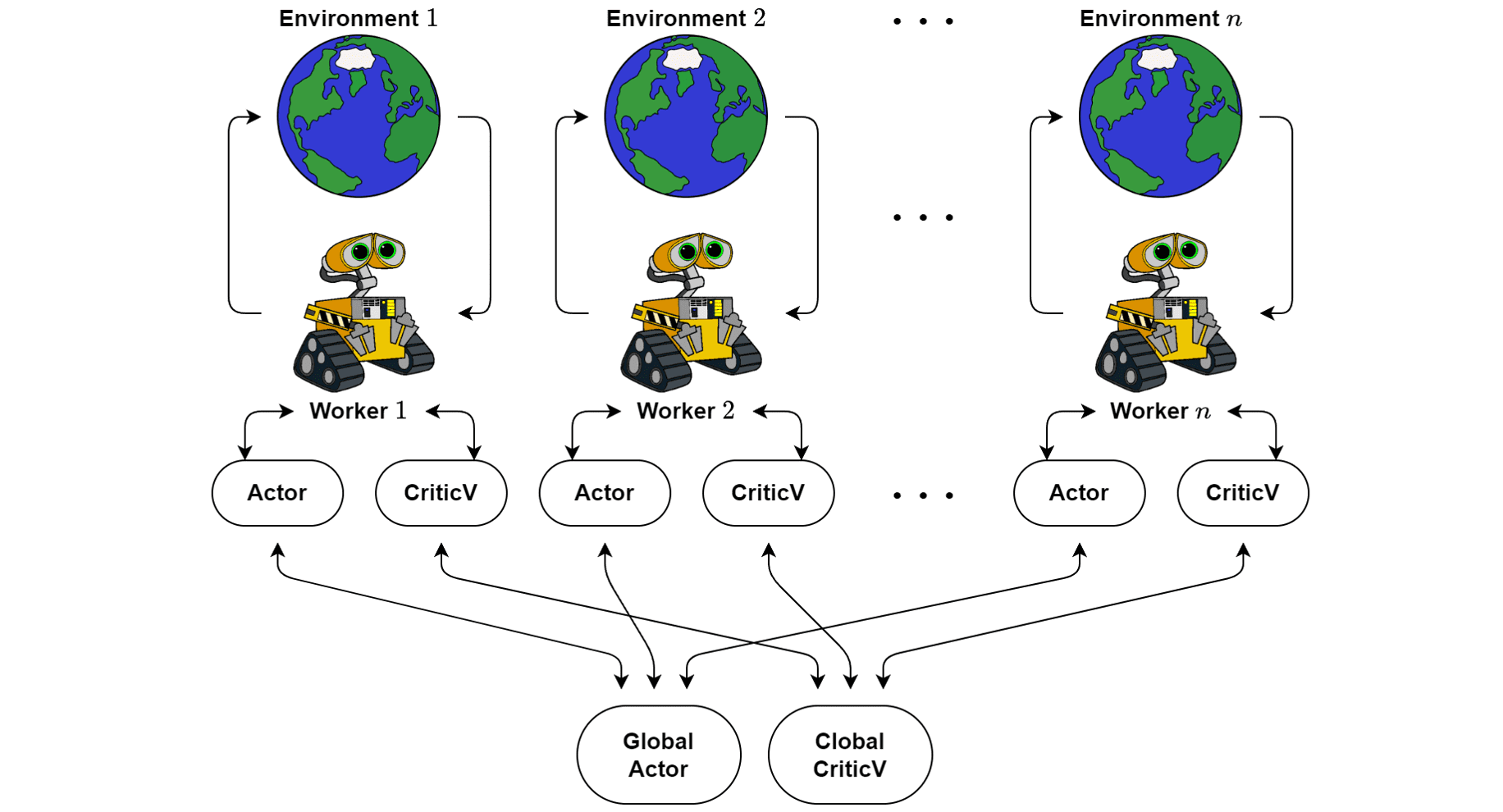
The policy and the value function are updated after every $t_{\textrm{max}}$ actions or when a terminal state is reached. The algorithm update each actor parameters via $\nabla_{\theta} \log \pi (\mathbf{a}_t \vert \mathbf{s}_t) \cdot A( \mathbf{s}_t, \mathbf{a}_t; \theta, \theta_v )$ where $A( \mathbf{s}_t, \mathbf{a}_t; \theta, \theta_v )$ is an estimate of the advantage function given by
\[A( \mathbf{s}_t, \mathbf{a}_t; \theta, \theta_v ) = \sum_{j=0}^{k-1} \gamma^j r_{t+j} + \gamma^k V_{\theta_v} (\mathbf{s}_{t+k}) - V_{\theta_v} (\mathbf{s}_t)\]where $k$ can vary from state to state and is upper-bounded by $t_{\max}$.
Off-policy Policy Gradient
So far, both REINFORCE and actor-critic methods are on-policy, meaning that training samples are collected according to the target policy that we aim to optimize. The off-policy methods provide several additional advantages.
-
The off-policy approach doesn’t necessitate full trajectories and can make use of any past episodes (through experience replay) for more efficient sample usage.
-
The sample collection follows a behavior policy that differs from the target policy, thereby enhancing exploration capabilities.
Let $\beta(\mathbf{a} \vert \mathbf{s})$ be a behavior policy and $\pi(\mathbf{a} \vert s)$ be a target policy. Then the objective function, the expected return of states, will be computed according to the distribution of state and action that is formed by behavior policy:
\[\begin{aligned} J(\theta)=\sum_{\mathbf{s} \in \mathcal{S}} d^\beta(\mathbf{s}) \sum_{\mathbf{a} \in \mathcal{A}} Q^\pi(\mathbf{s}, \mathbf{a}) \pi_\theta(\mathbf{a} \mid \mathbf{s})=\mathbb{E}_{s \sim d^\beta}\left[ \sum_{\mathbf{a} \in \mathcal{A}} Q^\pi(\mathbf{s}, \mathbf{a}) \pi_\theta(\mathbf{a} \mid \mathbf{s}) \right] \end{aligned}\]where $d^\beta (\mathbf{s}) = \underset{t \to \infty}{\text{ lim }} P(S_t = \mathbf{s} \vert S_0, \beta)$ is the stationary distribution of the behavior policy $\beta$. Hence, the policy gradient can be written as
\[\begin{aligned} \nabla_\theta J(\theta) & =\nabla_\theta \mathbb{E}_{\mathbf{s} \sim d^\beta}\left[\sum_{\mathbf{a} \in \mathcal{A}} Q^\pi(\mathbf{s}, \mathbf{a}) \pi_\theta(\mathbf{a} \mid \mathbf{s})\right] \\ & = \mathbb{E}_{\mathbf{s} \sim d^\beta}\left[\sum_{\mathbf{a} \in \mathcal{A}}\left(Q^\pi(\mathbf{s}, \mathbf{a}) \nabla_\theta \pi_\theta(\mathbf{a} \mid \mathbf{s}) + \color{red}{\pi_\theta(\mathbf{a} \mid \mathbf{s}) \nabla_\theta Q^\pi(\mathbf{s}, \mathbf{a})} \right) \color{black}{} \right] \end{aligned}\]by chain rule. However, in the red term, it is almost impossible to compute $\nabla_\theta Q^\pi (\mathbf{s}, \mathbf{a})$ when we don’t know what the target policy is. Fortunately, it turned out that the approximate gradient ignoring the red term still makes policy improvement, and thus guarateed to converge to true local minimum, by Degris, White and Sutton, 2012
Finally, we have
\[\begin{aligned} \nabla_\theta J(\theta) & = \mathbb{E}_{\mathbf{s} \sim d^\beta}\left[\sum_{\mathbf{a} \in \mathcal{A}}\left(Q^\pi(\mathbf{s}, \mathbf{a}) \nabla_\theta \pi_\theta(\mathbf{a} \mid \mathbf{s}) + \color{red}{\pi_\theta(\mathbf{a} \mid \mathbf{s}) \nabla_\theta Q^\pi(\mathbf{s}, \mathbf{a})}\right) \color{black}{} \right] \\ & \approx \mathbb{E}_{\mathbf{s} \sim d^\beta}\left[\sum_{\mathbf{a} \in \mathcal{A}} Q^\pi(\mathbf{s}, \mathbf{a}) \nabla_\theta \pi_\theta(\mathbf{a} \mid \mathbf{s}) \right] \\ & = \mathbb{E}_{\mathbf{s} \sim d^\beta}\left[\sum_{\mathbf{a} \in \mathcal{A}} \beta (\mathbf{a} \mid \mathbf{s}) \cdot \frac{\pi_\theta(\mathbf{a} \mid s)}{\beta( \mathbf{a} \mid \mathbf{s} )} Q^\pi(\mathbf{s}, \mathbf{a}) \frac{\nabla_\theta \pi_\theta(\mathbf{a} \mid \mathbf{s})}{\pi_\theta(\mathbf{a} \mid \mathbf{s})} \right] \\ & = \mathbb{E}_{\mathbf{s} \sim d^\beta}\left[\sum_{\mathbf{a} \in \mathcal{A}} \beta (\mathbf{a} \mid \mathbf{s}) \cdot \frac{\pi_\theta(\mathbf{a} \mid \mathbf{s})}{\beta( \mathbf{a} \mid \mathbf{s} )} Q^\pi(\mathbf{s}, \mathbf{a}) \nabla_\theta \text{ ln } \pi_\theta(\mathbf{a} \mid \mathbf{s}) \right] \\ & = \mathbb{E}_{\beta}\left[\color{blue}{\frac{\pi_\theta\left(\mathbf{a}_t \mid \mathbf{s}_t\right)}{\beta\left(\mathbf{a}_t \mid \mathbf{s}_t\right)} } \color{black}{} Q^\pi(\mathbf{s}, \mathbf{a}) \nabla_\theta \text{ ln } \pi_\theta(\mathbf{a} \mid \mathbf{s}) \right] \end{aligned}\]Thus, if one wants to apply policy gradient in the off-policy manner, one can simply multiply an importance weight to correct bias between target and behavior policy. In summary, the policy gradient of algorithms that we covered so far are outlined as below:
Natural Policy Gradient
When using the Euclidian metric $\lVert \boldsymbol{\theta} \rVert_2 = \sqrt{\boldsymbol{\theta}^\top \boldsymbol{\theta}}$, then the gradient varies for every parameterization $\boldsymbol{\theta}$ of the policy $\pi_{\boldsymbol{\theta}}$, which can lead to slow learning rates, even when employing higher-order gradient methods. This issue poses the question of whether we can achieve a covariant gradient descent, namely, a gradient descent that accounts for an invariant measure of the proximity between the current policy and the updated policy, based on the distribution of paths generated by each.
Kakade et al. NIPS 2001 is the first paper that tackled this challenge and suggested the natural gradient approach in the context of reinforcement learning:
\[\Delta \boldsymbol{\theta} = \gamma \mathbf{F}^{-1}(\boldsymbol{\theta}) \nabla_{\boldsymbol{\theta}} J(\boldsymbol{\theta})\]The concept has been extensively explored in Bagnell et al. (2003), Peters et al. (2003), and Peters et al. (2005). The primary theoretical advantage of this approach lies in its independence from the parameterization of the policy, making it applicable to arbitrary policies. As an example, see the following figure; we can observe that the natural gradient points the optimum point due to invariance to parameterization while the SGD fails since the scale of $\sigma$ dominates $k$. In practical terms, this leads to significantly faster convergence rates in most scenarios and reduces the need for manual parameter tuning of the learning algorithm. Please refer to these papers for detailed theoretical analysis.
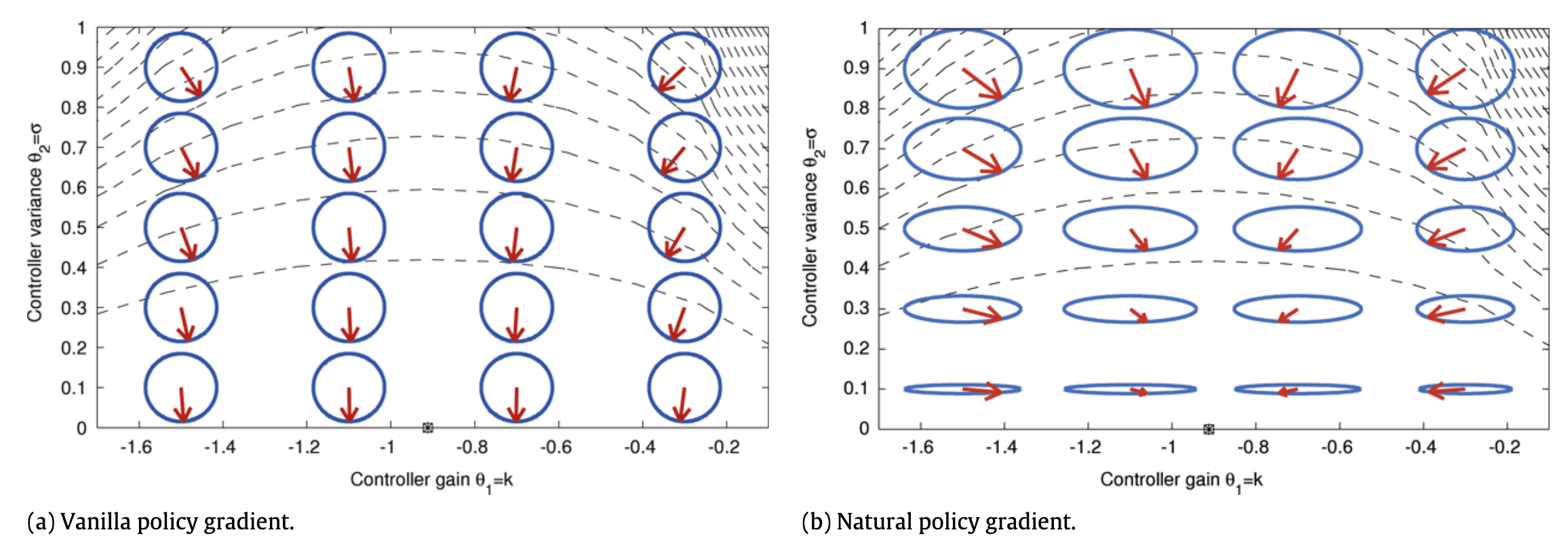
for parameterization: $\log \pi_\theta\left(\mathbf{a}_t \mid \mathbf{s}_t\right)=-\frac{1}{2 \sigma^2}\left(k \mathbf{s}_t-\mathbf{a}_t\right)^2+\mathrm{const} \quad \theta=(k, \sigma)$ where $r(\mathbf{s}_t, \mathbf{a}_t) = - \mathbf{s}_t^2 - \mathbf{a}_t^2$
Summary
Let me conclude the post by incorporating the practical advice of Sergey Levine, as shared in his CS285 at Berkeley, regarding the policy gradient methods:
- Remember that the gradient has high variance
- This isn’t the same as supervised learning!
- Gradients will be really noisy!
- Consider using much larger batches
- Tweaking learning rates is very hard
- Adaptive step size rules like ADAM can be OK-ish
Reference
[1] Reinforcement Learning: An Introduction. Richard S. Sutton and Andrew G. Barto, The MIT Press.
[2] Introduction to Reinforcement Learning with David Silver
[3] A (Long) Peek into Reinforcement Learning
[4] Going Deeper Into Reinforcement Learning: Fundamentals of Policy Gradients
[5] UC Berkeley, CS285, Deep Reinforcement Learning
[6] Foundations of Reinforcement Learning with Applications in Finance by Ashwin Rao
[7] Kakade et al., “A Natural Policy Gradient”, NIPS 2001
[8] Peters et al. (2008), “Reinforcement learning of motor skills with policy gradients”, Neural Networks
[9] Bagnell et al. “Covariant policy search”, In Proceedings of the international joint conference on artificial intelligence (pp. 1019–1024).
[10] Peters et al. (2003) “Reinforcement learning for humanoid robotics”, In Proceedings of the IEEE-RAS international conference on humanoid robots (HUMANOIDS) (pp. 103–123).
[11] Peters et al. (2005) “Natural actor-critic”. In Proceedings of the European machine learning conference (pp. 280–291).
[12] Will moving differentiation from inside, to outside an integral, change the result?
[13] Mnih et al. “Asynchronous Methods for Deep Reinforcement Learning”, ICML 2016
Leave a comment