[RL] Deep Policy Gradient

Trust Region Policy Optimization (TRPO)

Reinforcement Learning, especially policy gradient, is very sensitive to train in various aspects. So, it is good to update the policy carefully, which is often to change it by a small amount. Typically, this is done via gradient ascent (or descent) with small enough step size. However, this is done in parameter space but even seemingly small differences in parameter space can have very large differences in action space–so a single bad step can collapse the policy performance. The goal of TRPO is to avoid this kind of collapse.

Reinforcement Learning, particularly policy gradient methods, exhibit a high sensitivity during training across multiple aspects. Thus, it is required to update the policy cautiously, often with small amount of increments.

However, these adjustments occur within parameter space, where seemingly minor alterations can result in significant disparities within action space. Consequently, a single erroneous step may precipitate a collapse in policy performance. The objective of TRPO is to circumvent such collapses by employing strategies designed to ensure stability and robustness throughout the training process.

Policy Gradient as Policy Improvement

Examining the conceptual underpinnings of policy gradient, alternating between estimating advantage and improving policy, akin to the policy improvement algorithm in value-based methods. While immediately selecting the maximum advantage action in policy improvement, policy gradient adjusts its stochastic policy based on advantage estimations, thus offering a softened version of policy improvement.

From our original objective in policy gradient, i.e. the expected discounted reward

\[V(\theta) = \mathbb{E}_{\tau \sim p_{\theta}} \left[ \sum_{t=1} \gamma^t r(\mathbf{s}_t, \mathbf{a}_t) \right]\]

Kakade & Langford, 2002 have shown that the following identity holds:

$\color{red}{\mathbf{Thm.}}$ Policy Improvement of Policy Gradient
We have $$ V(\theta) - V(\theta_{\textrm{old}}) = \mathbb{E}_{\tau \sim p_{\theta} (\tau)} \left [ \sum_{t=1} \gamma^t A^{\pi_{\theta_{\textrm{old}}}} (\mathbf{s}_t, \mathbf{a}_t) \right] $$ where $\tau \sim p_{\theta} (\tau)$ indicates that actions are sample $\mathbf{a}_t \sim \pi_{\theta} (\cdot \vert \mathbf{s}_t)$: $$ \begin{aligned} p_\theta (\tau) & = p_\theta (\mathbf{s}_1, \mathbf{a}_1, \cdots, \mathbf{s}_T, \mathbf{a}_T) \\ & = p(\mathbf{s}_1) \prod_{t=1}^T \pi_\theta (\mathbf{a}_t \vert \mathbf{s}_t) \cdot p(\mathbf{s}_{t+1} \vert \mathbf{s}_t, \mathbf{a}_t) \end{aligned} $$

$\mathbf{Proof.}$

Note that \(V^{\pi_{\theta_{\textrm{old}}}} (\mathbf{s}_0)\) is a function of \(\mathbf{s}_0\). Thus, \(\mathbb{E}_{\mathbf{s}_0 \sim p (\mathbf{s}_0)} [V^{\pi_{\theta_{\textrm{old}}}} (\mathbf{s}_0)] = \mathbb{E}_{\tau \sim p_{\theta} (\tau)} [V^{\pi_{\theta_{\textrm{old}}}} (\mathbf{s}_0)]\). Then

\[\begin{aligned} V(\theta) - V(\theta_{\textrm{old}}) & = V(\theta) - \mathbb{E}_{\mathbf{s}_0 \sim p(\mathbf{s}_0)} \left[ V^{\pi_{\theta_{\textrm{old}}}} (\mathbf{s}_0) \right] \\ & = V(\theta) - \mathbb{E}_{\tau \sim p_{\theta} (\tau)} \left[V^{\pi_{\theta_{\textrm{old}}}} (\mathbf{s}_0) \right] \\ & = V(\theta) - \mathbb{E}_{\tau \sim p_{\theta} (\tau)} \left[ \sum_{t=0}^\infty \gamma^t V^{\pi_{\theta_{\textrm{old}}}} (\mathbf{s}_t) - \sum_{t=1}^\infty \gamma^t V^{\pi_{\theta_{\textrm{old}}}} (\mathbf{s}_t) \right] \\ & = V(\theta) + \mathbb{E}_{\tau \sim p_{\theta} (\tau)} \left[ \sum_{t=0}^\infty \gamma^t (\gamma V^{\pi_{\theta_{\textrm{old}}}} (\mathbf{s}_{t+1}) - V^{\pi_{\theta_{\textrm{old}}}} (\mathbf{s}_t))\right] \\ & = \mathbb{E}_{\tau \sim p_{\theta} (\tau)} \left[ \sum_{t=0}^\infty \gamma^t r(\mathbf{s}_t, \mathbf{a}_t) \right] + \mathbb{E}_{\tau \sim p_{\theta} (\tau)} \left[ \sum_{t=0}^\infty \gamma^t (\gamma V^{\pi_{\theta_{\textrm{old}}}} (\mathbf{s}_{t+1}) - V^{\pi_{\theta_{\textrm{old}}}} (\mathbf{s}_t))\right] \\ & = \mathbb{E}_{\tau \sim p_{\theta} (\tau)} \left[ \sum_{t=0}^\infty \gamma^t \times [ r(\mathbf{s}_t, \mathbf{a}_t) + \gamma V^{\pi_{\theta_{\textrm{old}}}} (\mathbf{s}_{t+1}) - V^{\pi_{\theta_{\textrm{old}}}} (\mathbf{s}_t)]\right] \\ & = \mathbb{E}_{\tau \sim p_{\theta} (\tau)} \left[ \sum_{t=0}^\infty \gamma^t A^{\pi_{\theta_{\textrm{old}}}} (\mathbf{s}_t, \mathbf{a}_t) \right] \end{aligned}\] \[\tag*{$\blacksquare$}\]

Kakade & Langford termed the RHS as policy advantage \(\mathbb{A}_{\pi_{\theta_{\textrm{old}}}} (\pi_\theta) = \mathbb{E}_{\tau \sim p_{\theta} (\tau)} [A^{\pi_{\theta_{\textrm{old}}}} (\mathbf{s}, \mathbf{a})]\), which quantifies the extent to which $\pi_{\theta}$ selects actions with large advantages with regard to the set of states visited under \(\pi_{\theta_{\textrm{old}}}\) starting from a state \(\mathbf{s}\). For example, note that \(\mathbb{E}_{\tau \sim p_{\theta} (\tau)} [A^{\pi_{\theta}} (\mathbf{s}_t, \mathbf{a}_t)]\), i.e. zero when \(\theta = \theta_{\textrm{old}}\). And also note that a policy found by one step of policy improvement maximizes this policy advantage since it updates the new policy by $\pi^\prime (\mathbf{s}) = \underset{\mathbf{a} \in \mathcal{A}}{\text{ arg max }} Q^\pi (\mathbf{s}, \mathbf{a})$.

Note that the RHS of the identity can be re-written with the (unnormalized) visitation frequencies at timestep $t$ when the agent follows the policy $\pi_{\theta}$, denoted as $\mathbb{P} (\mathbf{s}_t \vert \pi)$, as follows:

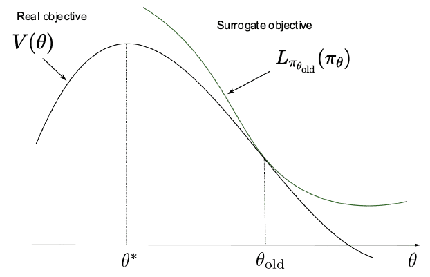
\[\begin{aligned} \mathbb{E}_{\tau \sim p_{\theta} (\tau)} \left[ \sum_{t=0}^\infty \gamma^t A^{\pi_{\theta_{\textrm{old}}}} (\mathbf{s}_t, \mathbf{a}_t) \right] & = \sum_{t=0}^{\infty} \sum_{\mathbf{s} \in \mathcal{S}} \mathbb{P} \left(\mathbf{s}_t= \mathbf{s} \mid \pi_{\theta} \right) \sum_{\mathbf{a} \in \mathcal{A}} \pi_{\theta} (\mathbf{a} \mid \mathbf{s}) \gamma^t A^{\pi_{\theta_{\textrm{old}}}}(\mathbf{s}, \mathbf{a}) \\ & = \sum_{t=0}^{\infty} \mathbb{E}_{\mathbf{s}_t \sim \mathbb{P} (\cdot \vert \pi_{\theta})} \left[ \mathbb{E}_{\mathbf{a}_t \sim \pi_{\theta} (\cdot \mid \mathbf{s})} \left[ \gamma^t A^{\pi_{\theta_{\textrm{old}}}}(\mathbf{s}_t, \mathbf{a}_t) \right] \right] \end{aligned}\]

Although the second expectation of \(\mathbf{a}_t \sim \pi_{\theta} (\cdot \mid \mathbf{s}_t)\) can be replaced by the old policy \(\pi_{\theta_{\textrm{old}}}\) with importance sampling, the challenge arises from the necessity to sample $(\mathbf{s}, \mathbf{a})$ from $\pi_{\theta}$, which remains unknown as $\pi_\theta$ is the target of our search. The basic idea of Kakade & Langford, 2002, which proposed conservative policy iteration (CPI), is to locally approximate this policy advantage by introducing the surrogate objective with the visitation frequency \(\mathbb{P} (\mathbf{s}_t \vert \pi_{\theta_{\textrm{old}}})\) rather than $\pi_{\theta}$:

\[V(\theta) \approx L_{\pi_{\theta_{\textrm{old}}}} (\pi_{\theta}) := V(\theta_{\textrm{old}}) + \sum_{t=0}^{\infty} \mathbb{E}_{\mathbf{s}_t \sim \mathbb{P} (\cdot \vert \pi_{\theta_{\textrm{old}}})} \left[ \mathbb{E}_{\mathbf{a}_t \sim \pi_{\theta} (\cdot \mid \mathbf{s}_t)} \left[ \gamma^t A^{\pi_{\theta_{\textrm{old}}}}(\mathbf{s}_t, \mathbf{a}_t) \right] \right]\]

Given that for any policy $\pi$, \(\mathbb{E}_{\tau \sim p_{\theta} (\tau)} [A^{\pi} (\mathbf{s}_t, \mathbf{a}_t)]\), note that for any parameter $\theta$

\[L_{\pi_{\theta}} (\pi_{\theta}) = V(\theta) \\ \left. \nabla_{\theta^\prime} L_{\pi_{\theta^\prime}} (\pi_{\theta^\prime}) \right\vert_{\theta^\prime = \theta} = \left. \nabla_{\theta^\prime} V(\theta^\prime) \right\vert_{\theta^\prime = \theta}\]

This implies that at least locally (i.e. $\Vert \theta - \theta_{\textrm{old}} \Vert \ll 1$), maximizing $L_{\pi_{\theta_{\textrm{old}}}} (\pi_{\theta})$ is equivalent to maximizing the true expected discounted reward $V(\theta)$.

$\mathbf{Fig\ 2.}$ Locally approximation with surrogate objective (Julien Vitay)

Trust Region Constraint

Then, how large a step size $\alpha$ is allowed for us to maximize $L_{\pi_{\theta_{\textrm{old}}}} (\pi_{\theta})$, ensuring the monotonic improvement of the policy? Schulman et al. ICML 2015 provided the theoretical inequality for measuring the quality of step size $\alpha$:

$\color{red}{\mathbf{Thm.}}$ Monotonic Improvement Guarantee
Denote $$ \textrm{KL}^{\max} (\pi_{\theta_{\textrm{old}}} \Vert \pi_{\theta_{\textrm{new}}}) = \underset{\mathbf{s} \in \mathcal{S}}{\max} \; \textrm{KL} (\pi_{\theta_{\textrm{old}}}( \cdot \vert \mathbf{s}) \Vert \pi_{\theta_{\textrm{new}}}( \cdot \vert \mathbf{s})) $$ For $\alpha = \textrm{KL}^{\max} (\pi_{\theta_{\textrm{old}}} \Vert \pi_{\theta_{\textrm{new}}}) $, then the following bound holds: $$ V(\theta_{\textrm{new}}) \geq L_{\pi_{\theta_{\textrm{old}}}} (\pi_{\theta_{\textrm{new}}}) - C \cdot \alpha \quad \text{ where } C =\frac{4\gamma \varepsilon}{1- \gamma} \text{ and } \varepsilon = \underset{\mathbf{s}, \mathbf{a} \in \mathcal{S} \times \mathcal{A}}{\max} A^{\pi_{\theta_{\textrm{old}}}} (\mathbf{s}, \mathbf{a}) $$

$\mathbf{Proof.}$

First, we can prove the similar inequality with total variance divergence, which is defined by

\[\textrm{TV} (\pi_{\theta_{\textrm{old}}}( \cdot \vert \mathbf{s}) \Vert \pi_{\theta_{\textrm{new}}}( \cdot \vert \mathbf{s})) = \frac{1}{2} \sum_{i=1}^{\vert \mathcal{A} \vert} \lvert \pi_{\theta_{\textrm{old}}}(\mathbf{a}_i \vert \mathbf{s}) - \pi_{\theta_{\textrm{new}}}(\mathbf{a}_i \vert \mathbf{s}) \rvert\]

for discrete probability distributions, i.e. discrete action space $\mathcal{A}$ instead of KL divergence:

$\color{green}{\mathbf{Lemma.}}$ Denote $$ \textrm{TV}^{\max} (\pi_{\theta_{\textrm{old}}} \Vert \pi_{\theta_{\textrm{new}}}) = \underset{\mathbf{s} \in \mathcal{S}}{\max} \; \textrm{TV} (\pi_{\theta_{\textrm{old}}}( \cdot \vert \mathbf{s}) \Vert \pi_{\theta_{\textrm{new}}}( \cdot \vert \mathbf{s})) $$ For $\alpha = \textrm{KL}^{\max} (\pi_{\theta_{\textrm{old}}} \Vert \pi_{\theta_{\textrm{new}}}) $, then the following bound holds: $$ V(\theta_{\textrm{new}}) \geq L_{\pi_{\theta_{\textrm{old}}}} (\pi_{\theta_{\textrm{new}}}) - C \cdot \alpha^2 \quad \text{ where } C =\frac{4\gamma \varepsilon}{(1- \gamma)^2} \text{ and } \varepsilon = \underset{\mathbf{s}, \mathbf{a} \in \mathcal{S} \times \mathcal{A}}{\max} A^{\pi_{\theta_{\textrm{old}}}} (\mathbf{s}, \mathbf{a}) $$

$\mathbf{Proof.}$

To bound the difference between $V(\theta)$ and $L_{\pi_{\theta_{\textrm{old}}}} (\pi_{\theta})$, we will bound the difference arising from each timestep. To do this, we first need to introduce a measure of how much $\pi_{\theta}$ and $\pi_{\theta_{\textrm{old}}}$ agree. For the local approximation, we will consider the policy $\pi_{\theta}$ that is proxy to $\pi_{\theta_{\textrm{old}}}$ with the following criteria:

\[\mathbb{P}(\mathbf{a}, \tilde{\mathbf{a}} \vert \mathbf{s}) \leq \alpha\]

where $(\mathbf{a}, \tilde{\mathbf{a}}) \sim \pi \times \tilde{\pi} \vert \mathbf{s}$, i.e. a joint distribution by $\pi (\cdot \vert \mathbf{s})$ and $\tilde{\pi} (\cdot \vert \mathbf{s})$.

Firstly, we can bound \(\mathbb{E}_{\mathbf{a}_t \sim \pi_{\theta} (\cdot \mid \mathbf{s}_t)} \left[ A^{\pi_{\theta_{\textrm{old}}}}(\mathbf{s}_t, \mathbf{a}_t) \right]\):

\[\begin{aligned} \mathbb{E}_{\tilde{\mathbf{a}} \sim \tilde{\pi}}\left[A^\pi(\mathbf{s}, \tilde{\mathbf{a}})\right] & = \mathbb{E}_{(\mathbf{a}, \tilde{\mathbf{a}}) \sim(\pi, \tilde{\pi})}\left[A^\pi(\mathbf{s}, \tilde{\mathbf{a}})-A^\pi(\mathbf{s}, \mathbf{a})\right] \quad \text { since } \quad \mathbb{E}_{\mathbf{a} \sim \pi}\left[A^\pi(\mathbf{s}, \mathbf{a})\right]=0 \\ & = \mathbb{P}(\mathbf{a} \neq \tilde{\mathbf{a}} \mid \mathbf{s}) \mathbb{E}_{(\mathbf{a}, \tilde{\mathbf{a}}) \sim(\pi, \tilde{\pi}) \mid \mathbf{a} \neq \tilde{\mathbf{a}}}\left[A^\pi(s, \tilde{\mathbf{a}})-A^\pi(\mathbf{s}, \mathbf{a})\right] \\ \mathbb{E}_{\tilde{\mathbf{a}} \sim \tilde{\pi}}\left[A^\pi(\mathbf{s}, \tilde{\mathbf{a}})\right] & \leq \alpha \cdot 2 \max _{\mathbf{s}, \mathbf{a}}\left|A^\pi(\mathbf{s}, \mathbf{a})\right| \end{aligned}\]

For brevity, let’s denote \(\bar{A}^{\pi_{\theta_\text{old}}}_{\pi_\theta} (\mathbf{s}_t) = \bar{A}^{\pi_{\theta_\text{old}}}_{\pi_\theta} (\mathbf{s}_t)\). Then, we will prove that an upper bound of the difference between the summand of policy advantage is given by:

\[\begin{aligned} & \left\vert \mathbb{E}_{\mathbf{s}_t \sim \mathbb{P} (\mathbf{s}_t \vert \pi_{\theta})} \left[ \mathbb{E}_{\mathbf{a}_t \sim \pi_{\theta} (\mathbf{a} \mid \mathbf{s})} \left[ A^{\pi_{\theta_{\textrm{old}}}}(\mathbf{s}, \mathbf{a}) \right] \right] - \mathbb{E}_{\mathbf{s}_t \sim \mathbb{P} (\mathbf{s}_t \vert \pi_{\theta_{\textrm{old}}})} \left[ \mathbb{E}_{\mathbf{a}_t \sim \pi_{\theta} (\mathbf{a} \mid \mathbf{s})} \left[ A^{\pi_{\theta_{\textrm{old}}}}(\mathbf{s}, \mathbf{a}) \right] \right] \right\vert \\ \leq & \; 2 \alpha \underset{\mathbf{s} \in \mathcal{S}} \max \mathbb{E}_{\mathbf{a}_t \sim \pi_{\theta} (\mathbf{a} \mid \mathbf{s})} \left[ A^{\pi_{\theta_{\textrm{old}}}}(\mathbf{s}, \mathbf{a}) \right] \\ \leq & \; 4\alpha (1 - (1 - \alpha)^t) \underset{\mathbf{s} \in \mathcal{S}} \max \vert A^{\pi_{\theta_{\textrm{old}}}} (\mathbf{s}, \mathbf{a}) \vert \end{aligned}\]

Let $n_t$ denote the number of times that $\mathbf{a}_i \neq \tilde{\mathbf{a}}_i$ for $i < t$, i.e., the number of times that $\pi$ and $\tilde{\pi}$ disagree before timestep $t$. By definition of $\alpha$, $P(n_t = 0) \geq (1 - \alpha)^t$ and $\mathbb{P} (n_t > 0) \leq 1 - (1 - \alpha)^t$. Then we can decompose the summand as follows:

\[\begin{aligned} \mathbb{E}_{\mathbf{s}_t \sim \mathbb{P} (\cdot \vert \pi_{\theta})} \left[ \bar{A}^{\pi_{\theta_\text{old}}}_{\pi_\theta} (\mathbf{s}_t) \right] & = \mathbb{P} (n_t = 0) \times \mathbb{E}_{\mathbf{s}_t \sim \mathbb{P} (\cdot \vert \pi_{\theta}) \vert n_t = 0} \left[ \bar{A}^{\pi_{\theta_\text{old}}}_{\pi_\theta} (\mathbf{s}_t) \right] \\ + & \; \mathbb{P} (n_t > 0) \times \mathbb{E}_{\mathbf{s}_t \sim \mathbb{P} (\cdot \vert \pi_{\theta}) \vert n_t > 0} \left[ \bar{A}^{\pi_{\theta_\text{old}}}_{\pi_\theta} (\mathbf{s}_t) \right] \\ \mathbb{E}_{\mathbf{s}_t \sim \mathbb{P} (\cdot \vert \pi_{\theta_{\textrm{old}}})} \left[ \bar{A}^{\pi_{\theta_\text{old}}}_{\pi_\theta} (\mathbf{s}_t) \right] & = \mathbb{P} (n_t = 0) \times \mathbb{E}_{\mathbf{s}_t \sim \mathbb{P} (\cdot \vert \pi_{\theta_{\textrm{old}}}) \vert n_t = 0} \left[ \bar{A}^{\pi_{\theta_\text{old}}}_{\pi_\theta} (\mathbf{s}_t) \right] \\ + & \; \mathbb{P} (n_t > 0) \times \mathbb{E}_{\mathbf{s}_t \sim \mathbb{P} (\cdot \vert \pi_{\theta_{\textrm{old}}}) \vert n_t > 0} \left[ \bar{A}^{\pi_{\theta_\text{old}}}_{\pi_\theta} (\mathbf{s}_t) \right] \\ \end{aligned}\]

Using that \(\mathbb{E}_{\color{blue}{\mathbf{s}_t \sim \mathbb{P} (\cdot \vert \pi_{\theta}) \vert n_t = 0}} \left[ \bar{A}^{\pi_{\theta_\text{old}}}_{\pi_\theta} (\mathbf{s}_t) \right] = \mathbb{E}_{\color{red}{\mathbf{s}_t \sim \mathbb{P} (\cdot \vert \pi_{\theta_{\text{old}}}) \vert n_t = 0}} \left[ \bar{A}^{\pi_{\theta_\text{old}}}_{\pi_\theta} (\mathbf{s}_t) \right]\), by subtracting the both equation we obtain:

\[\begin{aligned} & \mathbb{E}_{\mathbf{s}_t \sim \mathbb{P} (\cdot \vert \pi_{\theta})} \left[ \bar{A}^{\pi_{\theta_\text{old}}}_{\pi_\theta} (\mathbf{s}_t) \right] - \mathbb{E}_{\mathbf{s}_t \sim \mathbb{P} (\cdot \vert \pi_{\theta_{\textrm{old}}})} \left[ \bar{A}^{\pi_{\theta_\text{old}}}_{\pi_\theta} (\mathbf{s}_t) \right] \\ = & \; P(n_t > 0) \left( \mathbb{E}_{\mathbf{s}_t \sim \mathbb{P} (\cdot \vert \pi_{\theta}) \vert n_t > 0} \left[ \bar{A}^{\pi_{\theta_\text{old}}}_{\pi_\theta} (\mathbf{s}_t) \right] - \mathbb{E}_{\mathbf{s}_t \sim \mathbb{P} (\cdot \vert \pi_{\theta_{\textrm{old}}}) \vert n_t > 0} \left[ \bar{A}^{\pi_{\theta_\text{old}}}_{\pi_\theta} (\mathbf{s}_t) \right] \right) \\ \end{aligned}\]

By the following inequality (from the upper bound that we obtained in the first step):

\[\left\vert \mathbb{E}_{\mathbf{s}_t \sim \mathbb{P} (\cdot \vert \pi_{\theta}) \vert n_t > 0} \left[ \bar{A}^{\pi_{\theta_\text{old}}}_{\pi_\theta} (\mathbf{s}_t) \right] - \mathbb{E}_{\mathbf{s}_t \sim \mathbb{P} (\cdot \vert \pi_{\theta_{\textrm{old}}}) \vert n_t > 0} \left[ \bar{A}^{\pi_{\theta_\text{old}}}_{\pi_\theta} (\mathbf{s}_t) \right] \right\vert \leq 4\alpha \underset{\mathbf{s}, \mathbf{a} \in \mathcal{S} \times \mathcal{A}}{\max} \left\vert A^{\pi_{\theta_{\text{old}}}} (\mathbf{s}, \mathbf{a}) \right\vert\]

and the definition of $\alpha$, we finally get

\[\left\vert \mathbb{E}_{\mathbf{s}_t \sim \mathbb{P} (\cdot \vert \pi_{\theta})} \left[ \bar{A}^{\pi_{\theta_\text{old}}}_{\pi_\theta} (\mathbf{s}_t) \right] - \mathbb{E}_{\mathbf{s}_t \sim \mathbb{P} (\cdot \vert \pi_{\theta_{\textrm{old}}})} \left[ \bar{A}^{\pi_{\theta_\text{old}}}_{\pi_\theta} (\mathbf{s}_t) \right] \right\vert \leq 4\alpha (1 - (1 - \alpha)^t) \underset{\mathbf{s}, \mathbf{a} \in \mathcal{S} \times \mathcal{A}}{\max} \left\vert A^{\pi_{\theta_{\text{old}}}} (\mathbf{s}, \mathbf{a}) \right\vert\]

Now, we can bound the entire sum with the notation \(\varepsilon = \underset{\mathbf{s}, \mathbf{a} \in \mathcal{S} \times \mathcal{A}}{\max} \left\vert A^{\pi_{\theta_{\text{old}}}} (\mathbf{s}, \mathbf{a}) \right\vert\):

\[\begin{aligned} \vert V(\theta) - L_{\pi_{\theta_{\text{old}}}} (\pi_\theta) \vert & = \sum_{t=0}^\infty \gamma^t \left\vert \mathbb{E}_{\mathbf{s}_t \sim \mathbb{P} (\cdot \vert \pi_{\theta})} \left[ \bar{A}^{\pi_{\theta_\text{old}}}_{\pi_\theta} (\mathbf{s}_t) \right] - \mathbb{E}_{\mathbf{s}_t \sim \mathbb{P} (\cdot \vert \pi_{\theta_{\textrm{old}}})} \left[ \bar{A}^{\pi_{\theta_\text{old}}}_{\pi_\theta} (\mathbf{s}_t) \right] \right\vert \\ & \leq \sum_{t=0}^\infty \gamma^t \cdot 4 \alpha ( 1 - (1-\alpha)^t ) \varepsilon \\ & = 4\alpha \varepsilon \left( \frac{1}{1-\gamma} - \frac{1}{1 - \gamma (1-\alpha)} \right) \\ & = \frac{4\alpha^2 \gamma \varepsilon}{(1 - \gamma) (1 - \gamma (1-\alpha))} \\ & \leq \frac{4\alpha^2 \gamma \varepsilon}{(1 - \gamma)^2} \end{aligned}\]

The following useful proposition in Probability and Statistics theory proves our lemma:

Suppose $p_X$ and $p_Y$ are distributions with $\textrm{TV} (p_X \Vert p_Y) = \alpha$. Then, there exists a joint distribution $(X, Y)$ whose marginals are $p_X$, $p_Y$ such that $X = Y$ with probability $1 - \alpha$/

\[\tag*{$\blacksquare$}\]

Then, from the well-known inequality between total variance divergence and KL divergence (called Pinsker’s inequality):

\[\textrm{TV}(\mathbb{P} \Vert \mathbb{Q}) \leq \sqrt{2 \times \text{KL}(\mathbb{P} \Vert \mathbb{Q})}\]

the result naturally follows.

\[\tag*{$\blacksquare$}\]

It now follows from this inequality that the greedy update of policy

\[\pi_{i + 1} = \underset{\theta \in \mathcal{\Theta}}{\textrm{arg max}} \; \left\{ M_{i} (\theta) := L_{\pi_i} (\pi_{\theta}) - C \cdot \textrm{KL}^{\max} (\pi_i \Vert \pi_{\theta}) \right\}\]

with the notation $\pi_{i + 1} = \pi_{\theta_{i+1}}$, is guaranteed to generate a monotonically improving sequence of policies such that $V(\theta_{0}) \leq V(\theta_{1}) \leq V(\theta_{2}) \leq \cdots$. It is because

\[\begin{aligned} & V\left(\theta_{i+1} \right) \geq L_{\pi_i} (\pi_{i + 1}) - C \cdot \alpha \textrm{ by theorem, } \\ & \alpha = 0 \textrm{ if } \pi_{i + 1} = \pi_i, \textrm{ thus } V(\theta_i) = M_{i} (\theta_i), \\ & \therefore V\left(\theta_{i+1}\right)-V\left(\theta_i\right) \geq M_i\left(\theta_{i+1}\right)-M_i\left(\theta_i\right). \end{aligned}\]

Thus, by maximizing $M_i$ at each iteration, we guarantee that the true objective $V$ is non-decreasing. And trust region policy optimization (TRPO), which Schulman et al. ICML 2015 proposed, is an algorithm that practically approximates these updates with a constraint on the KL divergence rather than a penalty to robustly allow large updates.

Since maximization of objective with the penalty term $C \cdot \textrm{KL}^\max (\theta_{\textrm{old}}, \theta_{\textrm{new}})$ is possible to reduces the step size significantly (and also the computation of penalty term is not trivial), TRPO instead introduces the constraint on the KL divergence called trust region constraint to ensure the policy update within trust region:

\[\begin{aligned} & \operatorname*{maximize} \limits_{\theta \in \Theta} \; L_{\theta_{\text{old}}}(\theta) \\ & \text{subject to } \; \textrm{KL}^{\max} (\theta_{\text{old}}, \theta) \leq \delta. \end{aligned}\]

And TRPO further discards the intractable constraint of the boundness of KL divergence at every state in the state space, with heuristic approximation which considers the average KL divergence:

\[\begin{aligned} & \operatorname*{maximize} \limits_{\theta \in \Theta} \; L_{\theta_{\text{old}}}(\theta) \\ & \text{subject to } \; \mathbb{E}_{\mathbf{s} \sim \mathbb{P} (\mathbf{s} \vert \pi_{\theta_{\textrm{old}}})} \left[ \textrm{KL} (\pi_{\theta_{\text{old}}} (\cdot \vert \mathbf{s}) \; \Vert \; \pi_{\theta} (\cdot \vert \mathbf{s})) \right ] \leq \delta. \end{aligned}\]

Policy Optimization with Trust Region Constraint

To solve the trust region constrained optimization problem, TRPO approximates the objective with linear approximation:

\[L_{\theta_{\text{old}}}(\theta) \approx \nabla_{\theta} L_{\theta_{\text{old}}}(\theta)^\top (\theta - \theta_{\text{old}})\]

and KL divergence with quadratic approximation using the Fisher information matrix of $\pi_{\theta} (\cdot \vert \mathbf{s})$:

\[\begin{aligned} \mathbb{E}_{\mathbf{s} \sim \mathbb{P} (\mathbf{s} \vert \pi_{\theta_{\textrm{old}}})} \left[ \textrm{KL} (\pi_{\theta_{\text{old}}} (\cdot \vert \mathbf{s}) \; \Vert \; \pi_{\theta} (\cdot \vert \mathbf{s})) \right ] & \approx \frac{1}{2} \mathbb{E}_{\mathbf{s} \sim \mathbb{P} (\mathbf{s} \vert \pi_{\theta_{\textrm{old}}})} \left[ (\theta - \theta_{\text{old}})^\top \mathbf{F}(\theta_{\text{old}} \vert \mathbf{s}) (\theta - \theta_{\text{old}}) \right] \\ & := \frac{1}{2} (\theta - \theta_{\text{old}})^\top \bar{\mathbf{F}} (\theta_{\text{old}}) (\theta - \theta_{\text{old}}) \end{aligned}\]

where

\[\mathbf{F} (\theta \vert \mathbf{s}) = \mathbb{E}_{\mathbf{a} \sim \pi_{\theta} (\cdot \vert \mathbf{s})} \left[ \frac{\partial \log \pi_{\theta} (\mathbf{a} \vert \mathbf{s})}{\partial \theta} \frac{\partial \log \pi_{\theta} (\mathbf{a} \vert \mathbf{s})}{\partial \theta}^\top \right]\]

resulting in an approximate optimization problem that is exactly equivalent to the natural gradient formulation. (See my previous post of natural gradient.) Thus, by Lagrangian multiplier methods, we obtain

\[\theta_{k + 1} = \theta_k + \lambda \bar{\mathbf{F}} (\theta)^{-1} \nabla_{\theta} L_{\theta_{\text{old}}}(\theta).\]

And to satisfy the trust region constraint, the multiplier $\lambda$ is given by

\[\lambda = \sqrt{\frac{2 \delta}{\nabla_{\theta} L_{\theta_{\text{old}}}(\theta)^\top \bar{\mathbf{F}} (\theta)^{-1} \nabla_{\theta} L_{\theta_{\text{old}}}(\theta)}}\]

However, a challenge arises from the approximation errors inherent in the Taylor expansion, potentially leading to a violation of the KL constraint or a failure to enhance the surrogate advantage. To address this issue, TRPO incorporates a modification to the update rule: backtracking line search

\[\theta_{k+1} = \theta_k \alpha^j \sqrt{\frac{2 \delta}{\nabla_{\theta} L_{\theta_{\text{old}}}(\theta)^\top \bar{\mathbf{F}} (\theta)^{-1} \nabla_{\theta} L_{\theta_{\text{old}}}(\theta)}} \bar{\mathbf{F}} (\theta)^{-1} \nabla_{\theta} L_{\theta_{\text{old}}}(\theta)\]

where $\alpha \in (0, 1)$ is the backtracking coefficient, and \(j \in \mathbb{Z}_{\geq 0}\) such that $\pi_{\theta_{k+1}}$ satisfies the KL constraint and produces a positive surrogate advantage.

$\mathbf{Fig\ 3.}$ The pseudocode for TRPO algorithm (OpenAI)

Proximal Policy Optimization (PPO)

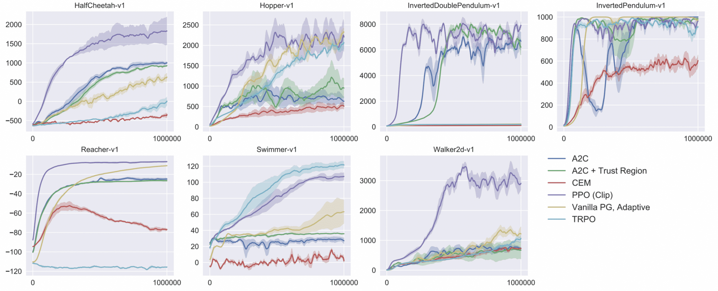
Solving the constrained optimization problem in TRPO makes the algorithm very complex. Proximal Policy Optimization (PPO) is a simplified alternative to TRPO, exhibiting comparable performance to TRPO in most scenarios.

Both TRPO and PPO grapple with a common motivation: how can we maximize policy improvement with high sample effciency; take cautious steps to circumvent performance collapse. While TRPO tackles this challenge with a sophisticated second-order approach, PPO adopts first-order optimizations augmented with additional strategies to ensure proximity between old and new policies.

From TRPO to PPO

If we denote the importance ratio as follows:

\[r_t (\theta) = \frac{\pi_\theta (\mathbf{a}_t \vert \mathbf{s}_t)}{\pi_{\theta_{\textrm{old}}} (\mathbf{a}_t \vert \mathbf{s}_t)}\]

the TRPO objective becomes

\[J^{\textrm{TRPO}} (\theta) = \mathbb{E}_{\tau \sim p_{\theta_{\textrm{old}}}} \left[ \frac{\pi_\theta (\mathbf{a}_t \vert \mathbf{s}_t)}{\pi_{\theta_{\textrm{old}}} (\mathbf{a}_t \vert \mathbf{s}_t)} \hat{A}^{\theta_{\textrm{old}}} (\mathbf{s}_t, \mathbf{a}_t) \right] = \mathbb{E}_{\tau \sim p_{\theta_{\textrm{old}}}} \left[ r_t (\theta) \hat{A}^{\theta_{\textrm{old}}} (\mathbf{s}_t, \mathbf{a}_t) \right]\]

where $\hat{A}$ is an estimator of the advantage function at timestep $t$. Then, the trust region constraint in PPO is simplified as follows:

\[J^{\textrm{CLIP}} (\theta) = \mathbb{E}_{\tau \sim p_{\theta_{\textrm{old}}}} \left[ \min \left\{ r_t (\theta) \hat{A}^{\theta_{\textrm{old}}} (\mathbf{s}_t, \mathbf{a}_t), \; \text{clip}(r_t (\theta), 1 - \epsilon, 1 + \epsilon) \hat{A}^{\theta_{\textrm{old}}} (\mathbf{s}_t, \mathbf{a}_t) \right\} \right]\]

where the function $\textrm{clip}()$ clips the ratio to be no more than $1 + \epsilon$ and no less than $1 - \epsilon$, where it’s kind of what KL term \(\mathbb{E}_{\mathbf{s} \sim \mathbb{P} (\mathbf{s} \vert \pi_{\theta_{\textrm{old}}})} [\textrm{KL} (\pi_{\theta_{\textrm{old}}} (\cdot \vert \mathbf{s}) \Vert \pi_{\theta} (\cdot \vert \mathbf{s}))] \leq \epsilon\) in TRPO does.

In addition to the clipped reward, the objective function is augmented with an error term on the value estimation (formula in red), a technique commonly utilized by most advantage-function estimators to reduce variance, and an entropy term (formula in blue) to encourage sufficient exploration.

\[L^{\textrm{CLIP}} (\theta) = \mathbb{E}_{\tau \sim p_{\theta_{\textrm{old}}}} \left[ J^{\textrm{CLIP}} (\theta) - \color{red}{c_1 (V_{\theta} (\mathbf{s}_t) - V_{\text{target}})^2 } + \color{blue}{c_2 \mathbb{H} (\mathbf{s}_t, \pi_{\theta} (\cdot \vert \mathbf{s}_t))} \right]\]

$\mathbf{Fig\ 4.}$ Comparison of several algorithms on several MuJoCo environments. With simple formulation, PPO outperforms TRPO in most environments. (Schulman et al. 2017)

Clipped Objective

The clipped objective in PPO ensures that the importance sampling weight remains close to $1$, thereby constraining the divergence between the new policy and the old one. Specifically,

• The advantage $\hat{A}^{\theta_{\textrm{old}}} (\mathbf{a}, \mathbf{s})$ is positive
  • the objective increase if the action becomes more likely, i.e. as $\pi_{\theta} (\mathbf{a} \vert \mathbf{s})$ increases
  • albeit $r_t (\theta) \geq 1 + \epsilon$, the objective is equally given as $(1 + \epsilon) \hat{A}^{\theta_{\textrm{old}}} (\mathbf{a}, \mathbf{s})$
  • therefore, the new policy does not gain advantage from deviating significantly from the old policy.
• The advantage $\hat{A}^{\theta_{\textrm{old}}} (\mathbf{a}, \mathbf{s})$ is negative
  • the objective increase if the action becomes less likely, i.e. as $\pi_{\theta} (\mathbf{a} \vert \mathbf{s})$ decreases
  • albeit $r_t (\theta) \leq 1 - \epsilon$, the objective is equally given as $(1 - \epsilon) \hat{A}^{\theta_{\textrm{old}}} (\mathbf{a}, \mathbf{s})$
  • therefore, the new policy does not gain advantage from deviating significantly from the old policy.

Reference

[1] Schulman et al. “Trust Region Policy Optimization”, ICML 2015
[2] OpenAI Spinning Up, “Trust Region Policy Optimization”
[3] Julien Vitay, “Natural gradients (TRPO, PPO)”
[4] Schulman et al. “Proximal Policy Optimization Algorithms”, arXiv preprint arXiv:1707.06347, 2017
[5] Lilian Weng, “Policy Gradient Algorithms”