
[RL] Model-Based Reinforcement Learning (MBRL)
Introduction
Sequential decision-making is a key challenge in the field of AI such as robotics, and two successful branches to solve this problem are planning and reinforcement learning. Planning, in this context, refers to any computational process that takes a model as input and produces or improves a policy for interacting with the modeled environment. Put simply, solving prediction/control using a model of the environment is known as planning the solution. This term originates from the fact that the AI agent predicts probabilistic scenarios of future states/rewards with the help of the model, for various choices of actions from specific states and solves for the necessary value function/policy based on the anticipated future outcomes projected from the model.
Even two ways are seemed to be different, the boundary of two methodologies do not need to be harsh; they can be integrated. Covering these methods, model-based reinforcement learning (MBRL) refers to any MDP approach that uses a model (known or learned) and plans to approximate a global value or policy function.
Such a model-based approach is usually not easy to optimize as we have to consider the model and value function simulateneously. Despite this difficulty, there are some advantages and reasons that model-based RL can be effective:
- models can efficiently learned by supervised learning methods;
- explicitly representing models can give us access to additional capabilities;
- use the learned models to represent uncertainty or to drive exploration.
- reduce the interactions in the real world;
- some interactions may be slow, inefficient, and dangerous in the real world.
- MBRL aligns with n analogy with human intelligence;
- human beings are capable of having an imagined world in mind, in which how things could happen following different actions can be predicted.
Definition of Model
Then, before we delve into the model-based learning, it is worth noting that what consitutes a model.
When provided with a state and an action, a model generates a prediction of the subsequent state and associated reward. In the case of a stochastic model, multiple potential next states and rewards exist, each with its own probability of occurrence. At this point, some models, which are referred to as distribution model, provide a description of all possible outcomes along with their respective probabilities, while sample model randomly select one outcome based on the probabilities for simulation. Obviously, distribution models are much stronger to learn and plan the world than sample models but in many applications it is much easier to obtain sample models.
Hence, a model $\mathcal{M}$ is a (approximate) representation of MDP \(\left\langle \mathcal{S}, \mathcal{A}, \mathcal{P}, \mathcal{R} \right\rangle\) where $\mathcal{S}$ and $\mathcal{A}$ denote the state space and action space, respectively, while $\mathcal{P}: \mathcal{S} \times \mathcal{A} \to \mathcal{S}$ and $\mathcal{R}: \mathcal{S} \times \mathcal{A} \to \mathbb{R}$ denotes the state transition dynamics and reward function, respectively. And normally, learning the model in MBRL corresponds to recovering the state transition dynamics $\mathcal{P}$ and the reward function $\mathcal{R}$.
Model Learning
The first component to consider is the learning of the environment model. At the early stage of RL research, the state and action spaces are finite and small, the model learning is sufficient to be considered with the tabular MDPs, where policies, transition dynamics, and reward functions can all be recorded in a table. And due to the advances of deep learning, now it is possible to accomodate dynamics of complex environments such as continuous states and actions.
World Model
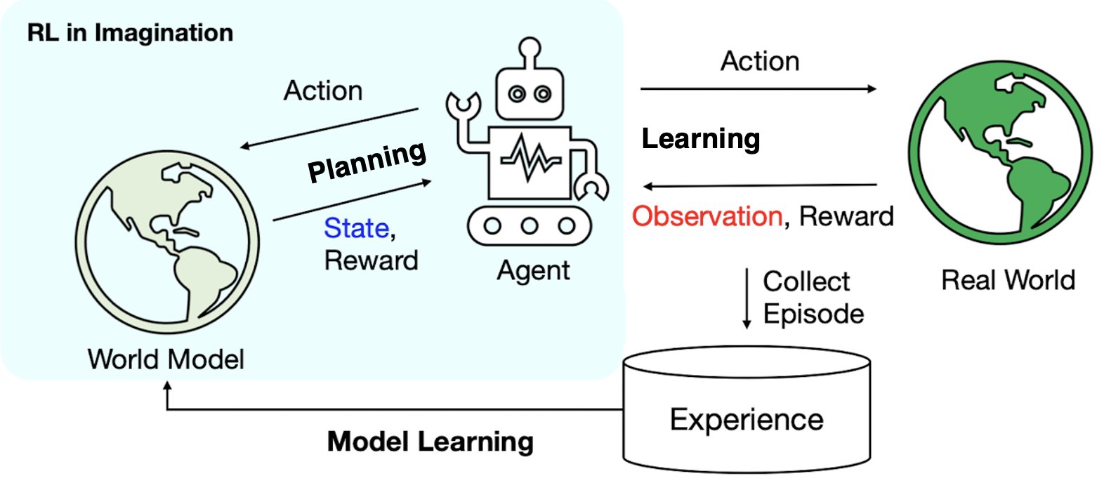
For high-dimensional state spaces such as images, representation learning that learns informative latent state or action representation proves invaluable for the environment model building, as it enhances the effectiveness and efficiency. Representatively, Ha & Schmidhuber et al. NIPS 2018 employed an autoencoder network to encode the latent state that can reconstruct the image, called world model.
World model learns a compressed spatial and temporal representation of the environment in an unsupervised manner. The features extracted from this learned world model are expressive to the point where an agent can train a highly compact and simple policy capable of solving the required task using the latent features. Remarkably, the agent can even training entirely within its own hallucinated dream, generated by its world model, and subsequently transfer this learned policy back into the actual environment.
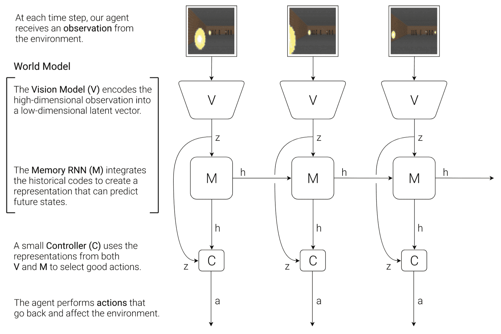
Inspired by human cognitive system, world model and its agent comprise of three components:
- Vision (V): visual sensory component
The vision (V) model learns an abstract, compressed representation $\mathbf{z}$ of each observed 2D image frame, using VAE framework. Hence, it is possible to generate the hallucinated environments from its latent vector.
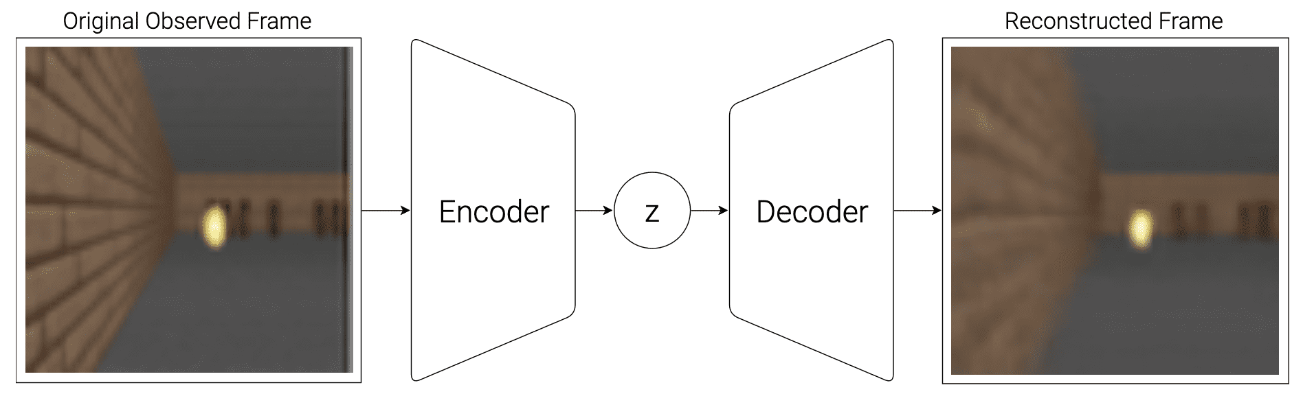
$\mathbf{Fig\ 3.}$ Flow diagram of V Model with VAE (Ha & Schmidhuber et al. 2018)
- Memory (M): memory component
The memory (M) model serves as a predictive model of the future $\mathbf{z}$ vectors that V is expected to produce. It hence can be viewed as the predictive and latent model of transition dynamics. Comprising an RNN that possesses memory of past in its hidden state $\mathbf{h}_t$, coupled with Mixture Density Newtork (MDN) to model $p (\mathbf{z}_{t+1} \vert \mathbf{a}_t, \mathbf{z}_t, \mathbf{h}_t)$, the M model efficiently captures the anticipated tranisition of environments.
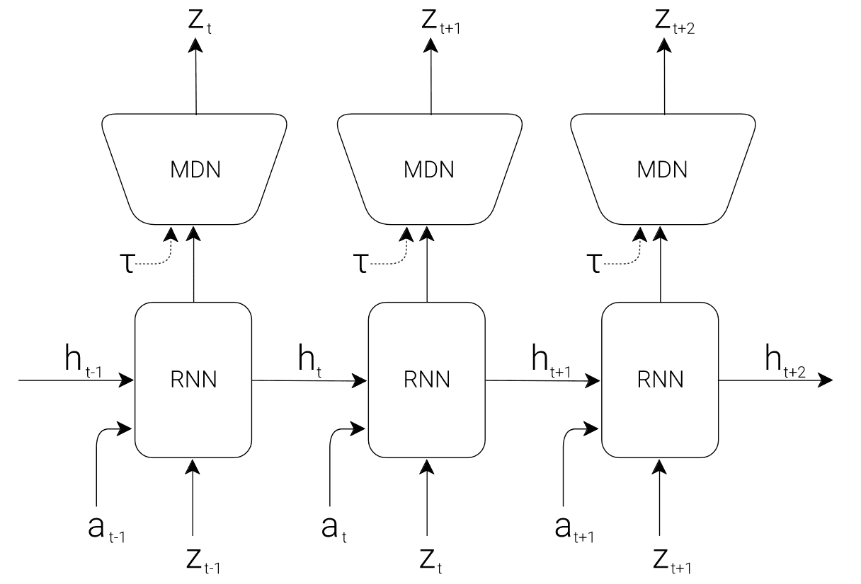
$\mathbf{Fig\ 4.}$ Flow diagram of M Model with RNN-MDN (Ha & Schmidhuber et al. 2018)
- Controller (C): decision-making component
Finally, the agent, controller (C) model determines the sequence of actions during the environment rollout. Leveraging the expressive capabilities and complexity of V & M models, the agent can be efficiently trained using a single-layer linear policy: $$ \mathbf{a}_t = \mathbf{W}_{\mathrm{c}} [\mathbf{z}_t ; \mathbf{h}_t] + \mathbf{b}_{\mathrm{c}} $$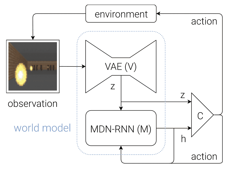
$\mathbf{Fig\ 5.}$ Flow diagram of the agent model (Ha & Schmidhuber et al. 2018)
Model Usage: Planning
Depending on the field of study and the specific applications, the interpretation of the term “planning” may vary. In the context of RL, planning typically denotes computational processes and algorithms that utilizes a model and generates a sequence of actions or refines policies by considering possible future situations within the modeled environment, devoid of direct interactions with the environment. And approaches for addressing RL challenges that leverage models and planning techniques are termed model-based methods.
Dynamic programming is actually a good example that we have already seen of a process that allows us to do planning. But, as the term planning implies, we’re generally interested in planning algorithms that don’t require privileged access to the specification of the world. One simple way is, we can just plug in a learned model in place of the privileged specification of the world in the dynamic programming.
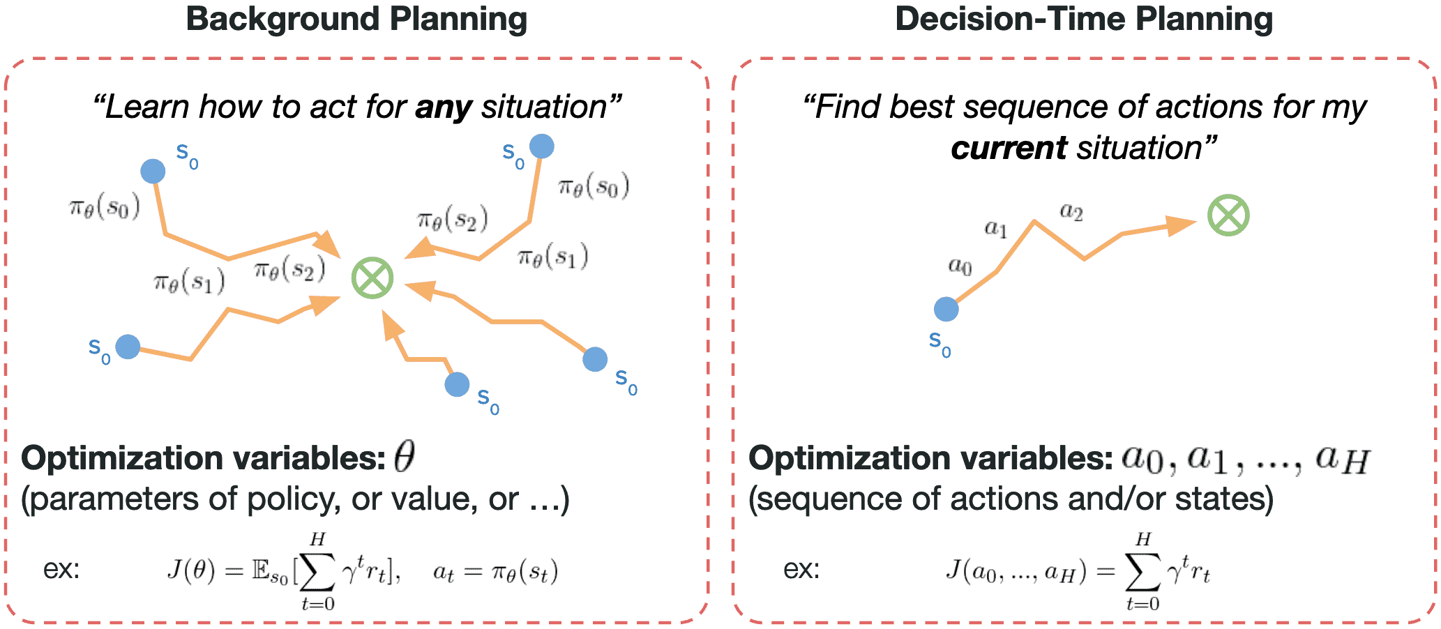
In MBRL, there aren’t a small number of easy-to-define clusters of methods for model-based RL: there are many orthogonal ways of using models. But it is frequently categorized into two different styles, decision-time planning and background planning. Like dynamic programming, it is possible to plan by continually improving a policy or value function on the basis of simulated experience from the model. Action selection is then quickly done by querying the approximated function at the current state. Such an approach of planning not focused on the current state is referred to as background planning. In contrast, decision-time planning focuses on a particular state and is performed as a computation whose output is the selection of a single action $a_t$ for the current state $s_t$; on the next step planning begins anew with $s_{t+1}$ to produce $a_{t+1}$, and so on.
Background Planning
Dyna-style Planning
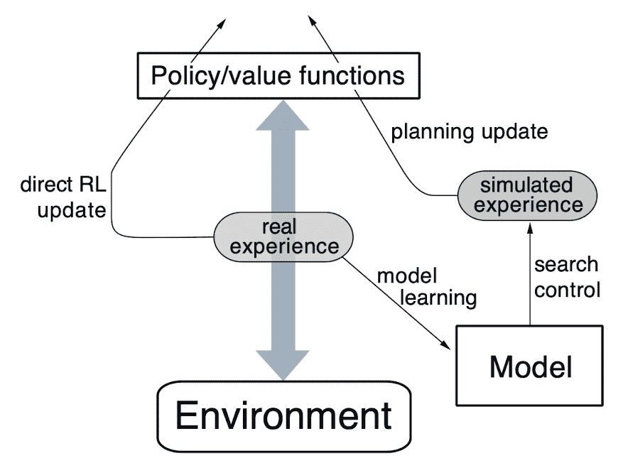
With a model, any number of simulated samples can be generated at will. Then, we can mix the real data with model-generated experience and apply traditional model-free algorithms like Q-learning, policy gradient, etc, resulting in a larger and augmented training dataset. These integrated approaches are known as Dyna-style methods. By treating real and simulated experience equivalently, they facilitate the learning and planning of value functions and policies from two distinct sources of experience data.
Since it is a general paradigm for integration of learning and planning, it can be incorporated into various algorithms and applied with diverse update rules to both simulated and real experiences.
Dyna-Q
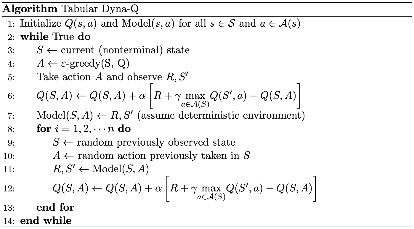
The simplest dyna-style method, Dyna-Q, as the name implies, is based on Q-learning for planning and learning. It assumes that the model is deterministic and model-learning is also table-based: records $(r_{t+1}, s_{t+1})$ in its table entry $(s_t, a_t)$. In other words, it simply predicts the next state and reward as the last-observed experience. (But also, function approximations such as deep neural networks instead of tabular setting can be employed to represent the value function/policy and the model.)
As an example, consider a simple maze where on each episode the agent starts on the initial state $S$ and \(\mathcal{A} = \{ \text{ up }, \text{ down }, \text{ left }, \text{ right } \}\). The dark cells are walls; if the agent tries to move into one of darker cells, then the action will have no effect. The agent can get reward only if it arrives in the goal state $G$.
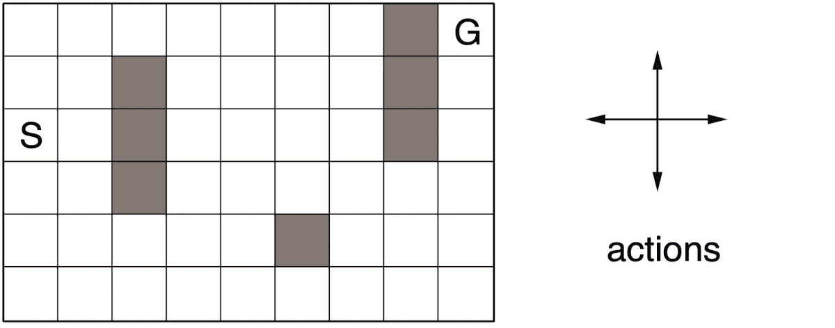
Note that that the Dyna-Q with $n = 0$ simply corresponds to the one-step tabular Q-Learning. By adding a planning for every real update, the agent manages to converge to the optimum much faster. And as $n$ increases, for instance to 50 planning steps, the agent actually converges in just a couple of episodes to the optimal policy.
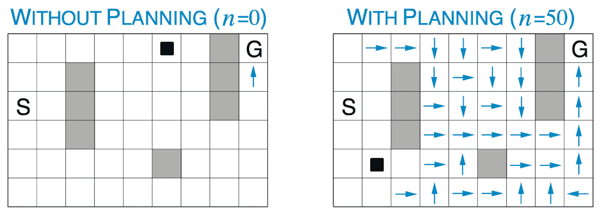
The next figure shows the reason for that. It displays the policies discovered by the agents with $n = 0$ and $n = 50$, respectively, reaching the midpoint of the second episode. The blue arrows indicates the greedy action in each state and thus no arrow in some states implies all of action values in that state were equal.
Dyna-Q+
However, in general, for instance in stochastic environment, models can be incorrect and non-generalizable, which is likely to converge to the local optimal policy. And in such scenarios the modeling error may not be detected for a long time, or forever.
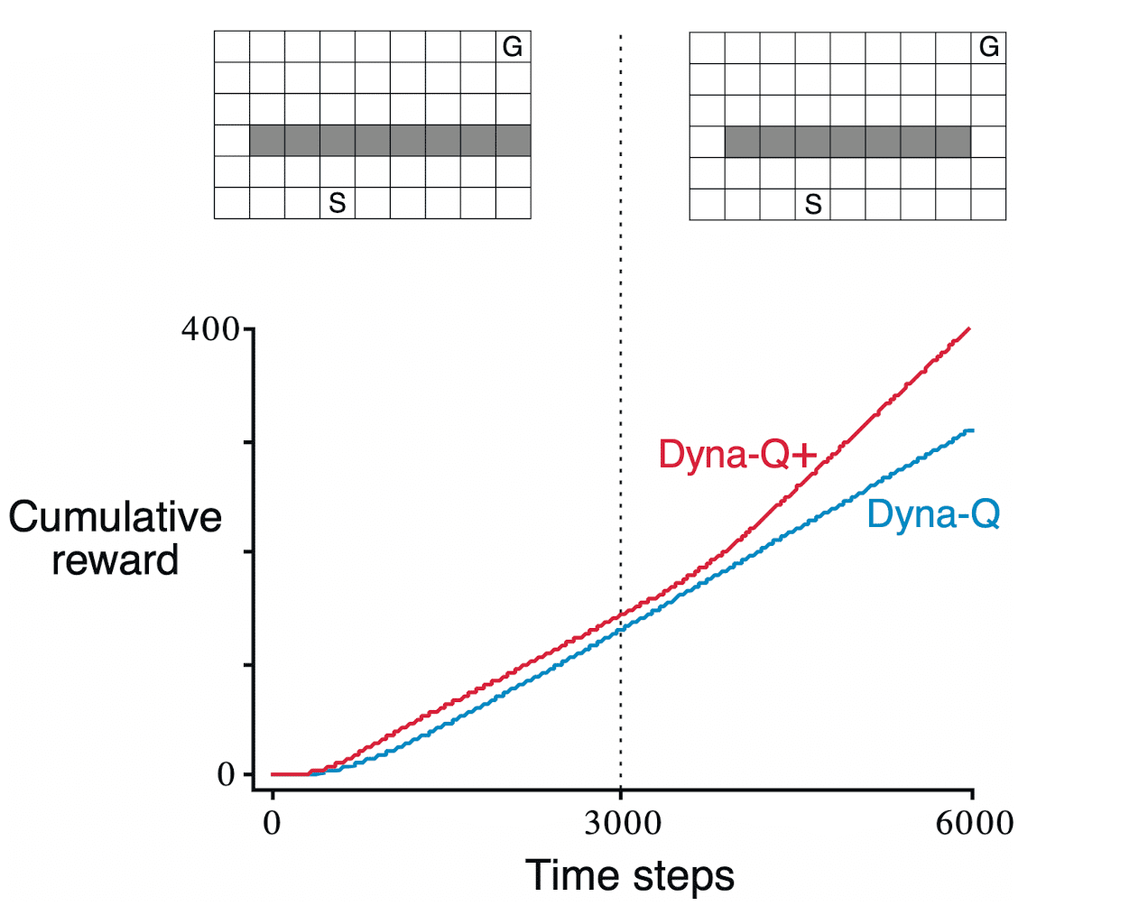
Let’s posit an initial scenario where the optimal path from the starting point to the goal is through the hole on the left side of the wall. However, after $3000$ time steps, suppose that the shortcut shifts as an additional hole is drilled on the right side of the wall.
The graph illustrates that the Dyna-Q agent maintains its initial understanding of the world, persisting with the established path. Consequently, as the agent engages in more planning, the probability of deviating to the right and discovering the shortcut diminishes. Even with an $\varepsilon$-greedy policy, it becomes highly improbable for the agent to take a substantial number of exploratory actions that would lead to the discovery of the shortcut situated on the opposite side.
To encourage the exploration of the agent, Dyna-Q+ adopts a simple heuristic:
the longer time that a state has been visited, the higher the likelihood that the dynamics of a particular state-action pair have altered, rendering the current model inaccurate.
To do so, for each state-action pair $(S, A)$, Dyna-Q+ agent keeps track of how many timesteps have elapsed since the pair $(S, A)$ was last visited in a real interaction with the environment, denoted as $\tau (S, A)$. And it grants a special bonus reward to actions that have been untried for a long period during simulated experiences that involve these actions:
\[\begin{aligned} Q(S, A) = Q(S, A)+\alpha\left[\left(R + \kappa \sqrt{\tau (S, A)} \right)+\gamma \underset{A \in \mathcal{A}}{\max} Q\left(S^{\prime}, A\right) -Q(S, A)\right] \end{aligned}\]where $R$ is the next reward with some small $\kappa$.
Model-Based Value Expansion (MBVE)
Under some conditions, Feinberg et al. 2018 shows that rolling out the model up to a fixed horizon $H$ and forming $H$-step TD targets (called $H$-step model value expansion):
\[\hat{V}_H (s_t) = \sum_{k = t}^{H + t - 1} \gamma^{k - t} \hat{r}_k + \gamma^H \hat{V}(\hat{s}_{t+H})\]can improve value estimates $\hat{V}$ of $V^\pi$ for a policy $\pi$, reducing the value estimation error
\[\underset{\nu}{\text{MSE}}(V) = \mathbb{E}_{S \sim \nu} [\lvert V(S) - V^\pi (S) \rvert^2]\]where $\nu$ is a distribution of states. Intuitively, $H$ serves as a measure of trust in the model, and controlling it allows for the management of model uncertainty.
Define $s_t$, $a_t$, $r_t$ to be the states, actions, and rewards resulting from following policy $\pi$ using the true dynamics $f: \mathcal{S} \times \mathcal{A} \to \mathcal{S}$ starting at $s_0 \sim v$ and analogously define $\hat{s}_t$, $\hat{a}_t$, $\hat{r}_t$ using the learned (or given) dynamics $\hat{f}: \mathcal{S} \times \mathcal{A} \to \mathcal{S}$ in place of $f$. Let the reward function $r$ be $L_r$-Lipschitz and the value function $V^\pi$ be $L_V$-Lipschitz. Let $\epsilon$ be an upper bound $$ \underset{t \in [H]}{\max} \mathbb{E} \lVert \hat{s}_t - s_t \rVert^2 \leq \epsilon $$ on the model risk for an $H$-step rollout. Then, for any parameterized value function $\hat{V}$, $H$-step model value expansion estimate $$ \hat{V}_H (s_t) = \sum_{k = t}^{H + t - 1} \gamma^{k - t} \hat{r}_k + \gamma^H \hat{V}(\hat{s}_{t+H}) $$ satisfies $$ \underset{\nu}{\operatorname{MSE}}(\hat{V}_H) \leq c_1^2 \epsilon^2+\left(1+c_2 \epsilon\right) \gamma^{2 H} \underset{(\hat{f^\pi})^H \nu}{\operatorname{MSE}}(\hat{V}) $$ where $c_1$, $c_2$ grow at most linearly in $L_r$, $L_V$ and are independent of $H$ for $\gamma < 1$, $(\hat{f^\pi})^H \nu$ denotes the pushforward measure resulting from playing $\pi$ $H$ times starting from states in $\nu$. We assume $\operatorname{MSE}_{(\hat{f^\pi})^H \nu} (\hat{V}) \geq 2$ for simplicity of presentation, but an analogous result holds when the critic outperforms the model.
Consider a random variable $X$ with probability measure $\lambda$, and put it through some transformation $f$. The distribution of the resulting random variable $f(X)$ is known as the pushforward distribution, or pushforward measure as the counterpart of distribution on the measure theory, defined by $f \mu = \mu \circ f^{-1}$.
The theorem implies that if $\epsilon$ is small and the value function $\hat{V}$ is at least as accurate on imagined states $(\hat{f^\pi})^H \nu$ as on those sampled from $\nu$:
\[\underset{\nu}{\operatorname{MSE}}(\hat{V}) \geq \underset{(\hat{f^\pi})^H \nu}{\operatorname{MSE}}(\hat{V})\]the MSE of the $H$-step value estimation will be approximately contracted by $\gamma^{2H}$:
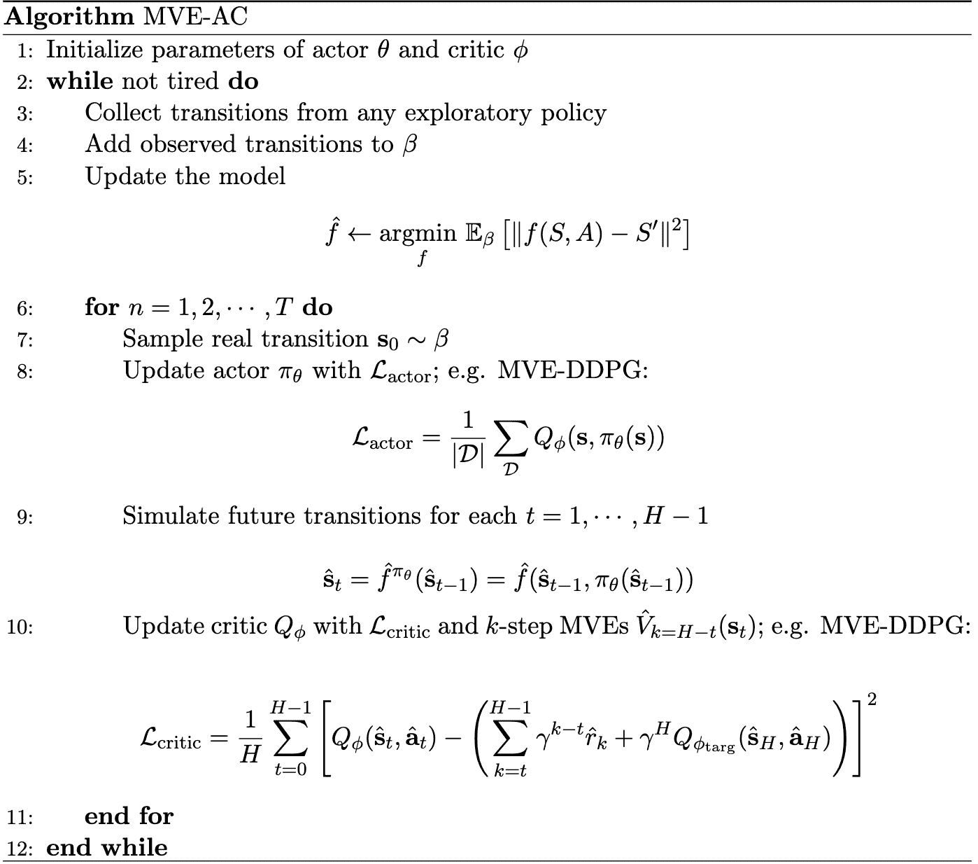
\[\begin{aligned} \underset{\nu}{\operatorname{MSE}}(\hat{V}_H) & \leq c_1^2 \epsilon^2+\left(1+c_2 \epsilon\right) \gamma^{2 H} \underset{(\hat{f^\pi})^H \nu}{\operatorname{MSE}}(\hat{V}) \\ & \leq c_1^2 \epsilon^2+\left(1+c_2 \epsilon\right) \gamma^{2 H} \underset{\nu}{\operatorname{MSE}}(\hat{V}) \approx \gamma^{2 H} \underset{\nu}{\operatorname{MSE}}(\hat{V}) \end{aligned}\]Moreover, to satisfy the condition \(\underset{\nu}{\operatorname{MSE}}(\hat{V}) \geq \underset{(\hat{f^\pi})^H \nu}{\operatorname{MSE}}(\hat{V})\), MVE enforce the training distribution $\nu$ to be a fixed point of $\hat{f^\pi}$, i.e. $(\hat{f^\pi})^H \nu = \nu$. Specifically, given an arbitrary off-policy distribution $\beta$ of state-action pair, set $\nu = \mathbb{E} [ (\hat{f^\pi})^T \beta ] = \frac{1}{H} \sum_{t=0}^{H - 1} (\hat{f^\pi})^t \beta$ as an approximation to the fixed point where $T \sim \mathcal{U} (0, \cdots, H-1)$.
MVE then samples a state $\hat{s}_T \vert T \sim (\hat{f^\pi})^T \beta$ and simulates $k = (H - T)$-step future transitions, training the critic $\hat{V} (\hat{s}_T)$ with $k$-step MVE targets $\hat{V}_k (\hat{s}_T)$. And in practice this simulation can be implemented by stratified sampling with $H$ dependent samples for each $t \in [H - 1]$.
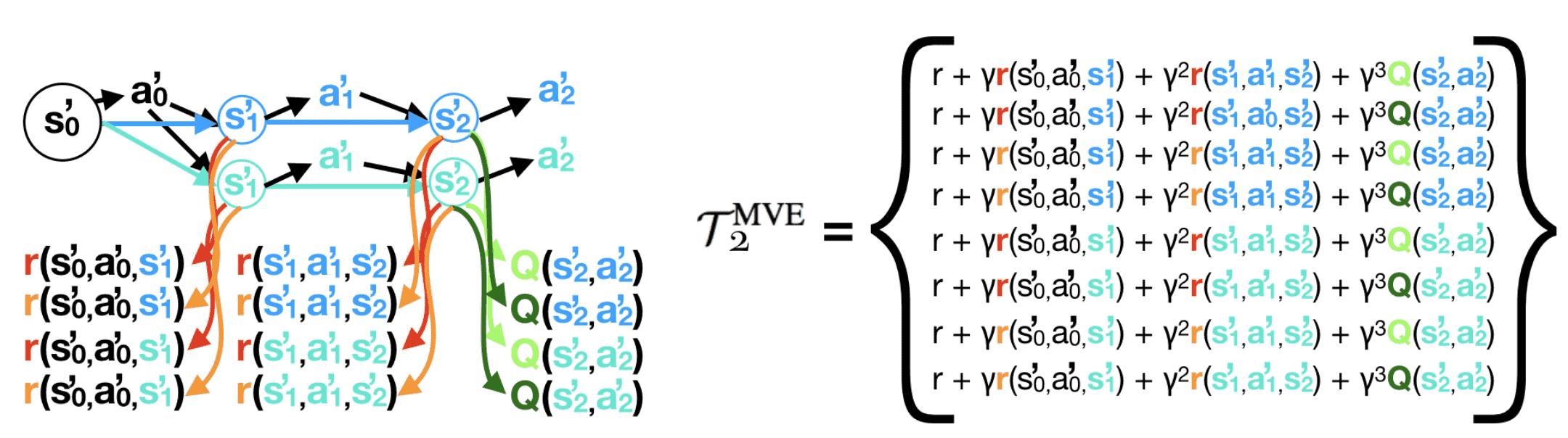
Stochastic Ensemble Value Expansion (STEVE)
MVE relies on fixed horizon $H$, which is task-specific and may change in different training phases and states space. Buckman et al. 2018 proposed an extension to MVE, called stochastic ensemble value expansion (STEVE), which further improves MVE by interpolating between many different horizon lengths $H$ based on the uncertainty calculated using ensemble. In ensembling, it prioritizes the rollout length with lower uncertainty by assigning a higher weight for weighted average.
Specifically, with $M$ dynamic models \(\{ \xi_1, \cdots, \xi_M \}\), $L$ critics \(\{ \theta_1, \cdots, \theta_L \}\), and $N$ reward models \(\{ \psi_1, \cdots, \psi_N \}\), STEVE rolls out an $H$ step trajectory from each model and denote \(\tau^{\xi_1}, \cdots, \tau_{\xi_M}\) where each trajectory consists of $H + 1$ states \(\hat{s}_0^{\xi_m}, \cdots \hat{s}_H^{\xi_m}\). Then, each model provides rollouts of various horizon lengths \(\{ \mathcal{T}_0^{\text{MVE}}, \cdots, \mathcal{T}_H^{\text{MVE}} \}\) where $\mathcal{T}_{\ell}^{\text{MVE}}$ denotes the MVE target with rollout horizon $\ell$:
\[\mathcal{T}_{\ell}^{\text{MVE}} (s_t) = \sum_{k = t}^{\ell + t - 1} \gamma^{k - t} \hat{r}_k + \gamma^\ell \hat{V}(\hat{s}_{t+\ell})\]Note that \(\mathcal{T}_0^{\text{MVE}}\) corresponds to vanilla TD target \(\mathcal{T}^{\text{TD}}\). For each rollout length $\ell$, we can compute the empirical mean and variance for each $\ell$-step MVE targets:
\[\begin{aligned} \mathcal{T}_\ell^\mu & = \frac{1}{M \cdot N \cdot L} \sum_{m = 1}^M \sum_{n=1}^N \sum_{l = 1}^L \mathcal{T}_{\ell, \xi_m, \psi_n, \theta_l}^{\text{MVE}} \\ \mathcal{T}_{\ell}^{\sigma^2} & = \frac{1}{M \cdot N \cdot L} \sum_{m = 1}^M \sum_{n=1}^N \sum_{l = 1}^L (\mathcal{T}_{\ell, \xi_m, \psi_n, \theta_l}^{\text{MVE}} - \mathcal{T}_\ell^\mu)^2 \end{aligned}\]and construct the STEVE target as follows:
\[\mathcal{T}_H^{\text{STEVE}} = \sum_{\ell=0}^{H} \frac{w_\ell}{\sum_{j} w_j} \mathcal{T}_\ell^\mu \quad \text{ where } \quad w_\ell = \frac{1}{\mathcal{T}_{\ell}^{\sigma^2}}\]where $w_\ell$ is set to minimize the MSE between the weighted-average of MVE targets and the true Q-value.
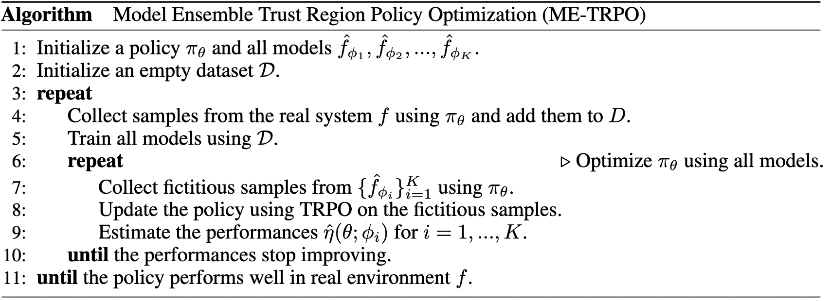
Model Ensemble Trust Region Policy Optimization (ME-TRPO)
Instead of value estimation, planning can also be used by model-free RL methods for policy improvement. In this case, the learned dynamic model can be regarded as a simulator where the policy can be trained. Representatively, model ensemble trust region policy optimization (ME-TRPO) introduced by Kurutach et al. 2018 learns a policy via TRPO from a set of learned models.
The standard approach for model-based policy learning alternates between model learning of $\hat{f_\phi}$ and policy optimization of $\pi_{\theta}$:
-
Model Learning
\[\phi^* = \underset{\phi}{\text{argmin}} \frac{1}{\vert \mathcal{D} \vert} \sum_{(\mathbf{s}_t, \mathbf{a}_t, \mathbf{s}_{t+1}) \in \mathcal{D}} \lVert \mathbf{s}_{t+1} - \hat{f_\phi} (\mathbf{s}_t, \mathbf{a}_t) \rVert^2\] -
Policy Optimization via policy gradient $\theta \leftarrow \theta + \nabla_{\theta} J(\theta, \phi)$ where
\[\nabla_{\theta} J(\theta, \phi) = \mathbb{E}_{\mathbf{s}_0 \sim \rho, \mathbf{a}_t \sim \pi_{\theta} (\cdot \vert \mathbf{s}_t), \mathbf{s}_{t+1} \sim \hat{f_\phi} (\mathbf{s}_t, \mathbf{a}_t)} \left[ \left(\sum_{t=0}^T \nabla_\theta \text{ log } \pi_\theta (\mathbf{a}_t \vert \mathbf{s}_t) \right) \left(\sum_{t=0}^T r(\mathbf{s}_t, \mathbf{a}_t)\right) \right]\]
The policy learning approaches that exploit the policy gradient theorem is also known as likelihood-ratio methods due to the usage of likelihood-ratio gradient $\nabla_\theta p_\theta (\tau) = p_\theta (\tau) \nabla_\theta \text{ log } p_\theta (\tau)$. Since MBRL framework requires backpropagation through time (BPTT) that multiplies many Jacobian, which is prone to vanishing/exploding gradient, the likelihood-ratio methods are generally employed to circumvent BPTT.
However, the learned policy frequently overfits, particularly by exploiting areas where training data for the dynamics model is scarcely available. Since we are improving the policy with respect to the approximate dynamics $\hat{f}$ instead of the real dynamics $f$, the predictions then can be erroneous and the errors may be accumulated. To mitigate this issue, ME-TRPO adopts the model ensemble of a set of dynamics models \(\{ \hat{f_{\phi_1}}, \cdots, \hat{f_{\phi_K}} \}\) as the regularization. In every step, a model $\hat{f_{\phi}}$ is randomly selected to predict the next state given the current state and action. And after every 5 gradient updates, it validates the policy’s performance using the $K$ learned model:
\[\frac{1}{K} \sum_{k=1}^K \boldsymbol{1} [ J (\theta_{\textrm{new}}, \phi_{k}) > J (\theta_{\textrm{old}}, \phi_{k})]\]and stops improvement if this ratio falls below the threshold $70\%$.
End-to-End Training with Models
In many MBRL scenarios, the dynamic models are typically modeled to be differentiable such as neural networks. Leveraging the internal architecture of these differentiable models enables seamless integration of planning or learning policy by interlinking the policy, model, and reward function. This allows the computation of an analytic policy gradient end-to-end, accomplished through backpropagation of rewards along a trajectory.
\[\begin{gathered} J(\theta) = \sum_{t=1}^T \gamma^t r (\mathbf{s}_t, \mathbf{a}_t) \text{ where } \mathbf{a}_t = \pi_{\theta} (\mathbf{s}_t) \text{ and } \mathbf{s}_t = f_\phi (\mathbf{s}_{t-1}, \mathbf{a}_{t-1}) \\ \Downarrow \\ \nabla_{\theta} J(\theta) = \sum_{t=1}^T \gamma^t \nabla_{\mathbf{s}_t} r(\mathbf{s}_t, \mathbf{a}_t) \nabla_{\phi} f_\phi (\mathbf{s}_{t-1}, \mathbf{a}_{t-1}) + \gamma^t \nabla_{\mathbf{a}_t} r(\mathbf{s}_t, \mathbf{a}_t) \nabla_{\theta} \pi_{\theta} (\mathbf{s}_t) \\ \nabla_{\phi} f_\phi (\mathbf{s}_{t-1}, \mathbf{a}_{t-1}) = \nabla_{\mathbf{s}_{t-1}} f_{\phi}(\mathbf{s}_{t-1}, \mathbf{a}_{t-1}) \nabla_{\phi} f_\phi (\mathbf{s}_{t-2}, \mathbf{a}_{t-2}) + \nabla_{\mathbf{a}_{t-1}} f_{\phi}(\mathbf{s}_{t-1}, \mathbf{a}_{t-1}) \nabla_{\theta} \pi_\theta (\mathbf{s}_{t-1}) \end{gathered}\]However, since it requires successive multiplication of Jacobians due to recursive differentiation (BPTT), which is prone to vanishing/exploding gradient. Instead of using entire trajectories, one can estimate future rewards using a learned value function (a critic) and compute policy gradients from subsequences of trajectories.
Stochastic Value Gradient (SVG)
For deterministic model $\mathbf{s}_{t+1} = f(\mathbf{s}_t, \mathbf{a}_t)$, differentiating the deterministic Bellman equation yields an expression for the value gradient of critic $V$:
\[\begin{aligned} \nabla_{\theta} V (\mathbf{s}_t) & = \nabla_{\theta} \left[ r(\mathbf{s}_t, \mathbf{a}_t) + \gamma V (\mathbf{s}_{t+1}) \right] \\ & = \nabla_{\mathbf{a}_t} r(\mathbf{s}_t, \mathbf{a}_t) \nabla_{\theta} \mathbf{a}_t + \gamma \nabla_{\theta} V (\mathbf{s}_{t+1}) + \gamma \nabla_{\mathbf{s}_{t+1}} V (\mathbf{s}_{t+1}) \nabla_{\mathbf{a}} f(\mathbf{s}_t, \mathbf{a}_t) \nabla_{\theta} \pi_{\theta} (\mathbf{s}_t) \\ \nabla_{\mathbf{s}_t} V (\mathbf{s}_t) & = \nabla_{\mathbf{s}_t} \left[ r(\mathbf{s}_t, \mathbf{a}_t) + \gamma V (\mathbf{s}_{t+1}) \right] \\ & = \nabla_{\mathbf{s}_t} r(\mathbf{s}_t, \mathbf{a}_t) + \nabla_{\mathbf{a}_t} r(\mathbf{s}_t, \mathbf{a}_t) \nabla_{\mathbf{s}_t} \pi_{\theta} (\mathbf{s}_t) + \gamma \nabla_{\mathbf{s}_{t+1}} V(\mathbf{s}_{t+1}) \left\{ \nabla_{\mathbf{s}_t} f(\mathbf{s}_t, \mathbf{a}_t) + \nabla_{\mathbf{a}_t} f(\mathbf{s}_t, \mathbf{a}_t) \nabla_{\mathbf{s}_t} \pi_{\theta} (\mathbf{s}_t) \right\} \end{aligned}\]Heess et al. 2015 first proposed the value gradient method that supports stochastic control, called stochastic value gradient (SVG). It extends the deterministic behavior of value gradient to stochastic, by treating stochasticity in the Bellman equation as a deterministic function of exogenous noise.
Particularly, SVG re-parameterize the stochastic policy $\pi_{\theta} (\mathbf{a} \vert \mathbf{s})$ and stochastic dynamics $f_{\phi} (\mathbf{s}, \mathbf{a})$ by regarding the policy and model as deterministic function $\pi_{\theta}$, $f_{\phi}$ of state $\mathbf{s}$, action $\mathbf{a}$ and noises $\eta$, $\xi$:
\[\begin{gathered} \mathbf{a} = \pi_{\theta} (\mathbf{s}, \eta) \\ \mathbf{s}^\prime = f_\phi (\mathbf{s}, \mathbf{a}, \xi) \end{gathered}\]where $\eta \sim \rho (\eta)$ and $\xi \sim \rho (\xi)$, respectively. Then, the true value function $V^\pi (\mathbf{s}_t)$ can be estimated by $H$-step return with our critic $V$ with the stochastic Bellman equation:
\[\begin{gathered} V^\pi (\mathbf{s}_t) \approx V (\mathbf{s}_t) = \mathbb{E}_{\eta \sim \rho(\eta)} \left[ r (\mathbf{s}_t, \mathbf{a}_t) + \gamma \mathbb{E}_{\xi \sim \rho (\xi)} \left[ V(\mathbf{s}_{t + 1}) \right] \right] \\ \text{ where } \mathbf{a}_{t} = \pi_{\theta} (\mathbf{s}_t, \eta_t), \quad \mathbf{s}_{t+1} = f_{\phi} (\mathbf{s}_t, \mathbf{a}_t, \xi_t) = f_{\phi} ( f_{\phi} (\mathbf{s}_{t-1}, \mathbf{a}_{t-1}, \xi_t), \pi_{\theta} (\mathbf{s}_t, \eta_t), \xi_{t-1} ) = \cdots \end{gathered}\]Differentiating the equation with respect to the current state $\mathbf{s}_t$ and policy parameters $\theta$ provides
\[\begin{aligned} \nabla_{\mathbf{s}_t} V(\mathbf{s}_t) = & \; \mathbb{E}_{\eta \sim \rho(\eta)} [ \nabla_{\mathbf{s}_t} r (\mathbf{s}_t, \mathbf{a}_t) + \nabla_{\mathbf{a}_t} r (\mathbf{s}_t, \mathbf{a}_t) \nabla_{\mathbf{s}_t} \pi_{\theta} (\mathbf{s}_t, \eta_t) \\ & + \gamma \mathbb{E}_{\xi \sim \rho (\xi)} \left[ \nabla_{\mathbf{s}_{t+1}} V(\mathbf{s}_{t + 1}) \cdot \left\{ \nabla_{\mathbf{s}_t} f_{\phi} (\mathbf{s}_t, \mathbf{a}_t, \xi_t) + \nabla_{\mathbf{a}_t} f_{\phi} (\mathbf{s}_t, \mathbf{a}_t, \xi_t) \nabla_{\mathbf{s}_t} \pi_{\theta} (\mathbf{s}_t, \eta_t) \right\} \right] ] \\ \nabla_{\theta} V(\mathbf{s}_t) = & \; \mathbb{E}_{\eta \sim \rho(\eta)} [ \nabla_{\mathbf{a}_t} r (\mathbf{s}_t, \mathbf{a}_t) \nabla_{\theta} \pi_{\theta} (\mathbf{s}_t, \eta_t) \\ & + \gamma \mathbb{E}_{\xi \sim \rho (\xi)} \left[ \nabla_{\mathbf{s}_{t+1}} V(\mathbf{s}_{t + 1}) \cdot \nabla_{\mathbf{a}_t} f_{\phi} (\mathbf{s}_t, \mathbf{a}_t, \xi_t) \nabla_{\theta} \pi_{\theta} (\mathbf{s}_t, \eta_t) + \nabla_{\theta} V(\mathbf{s}_{t + 1}) \right] ] \\ \end{aligned}\]Then, as a usual planning method, we sample a trajectory $\tau = (\mathbf{s}_1, \eta_1, \mathbf{a}_1, \xi_1, \mathbf{s}_2, \eta_2, \mathbf{a}_2, \xi_2, \cdot )$, and Monte-Carlo estimate of the policy gradient can be computed by the backward recursions on this sampled trajectory. For instance, in the original paper, one-sample estimates of gradients are given by:
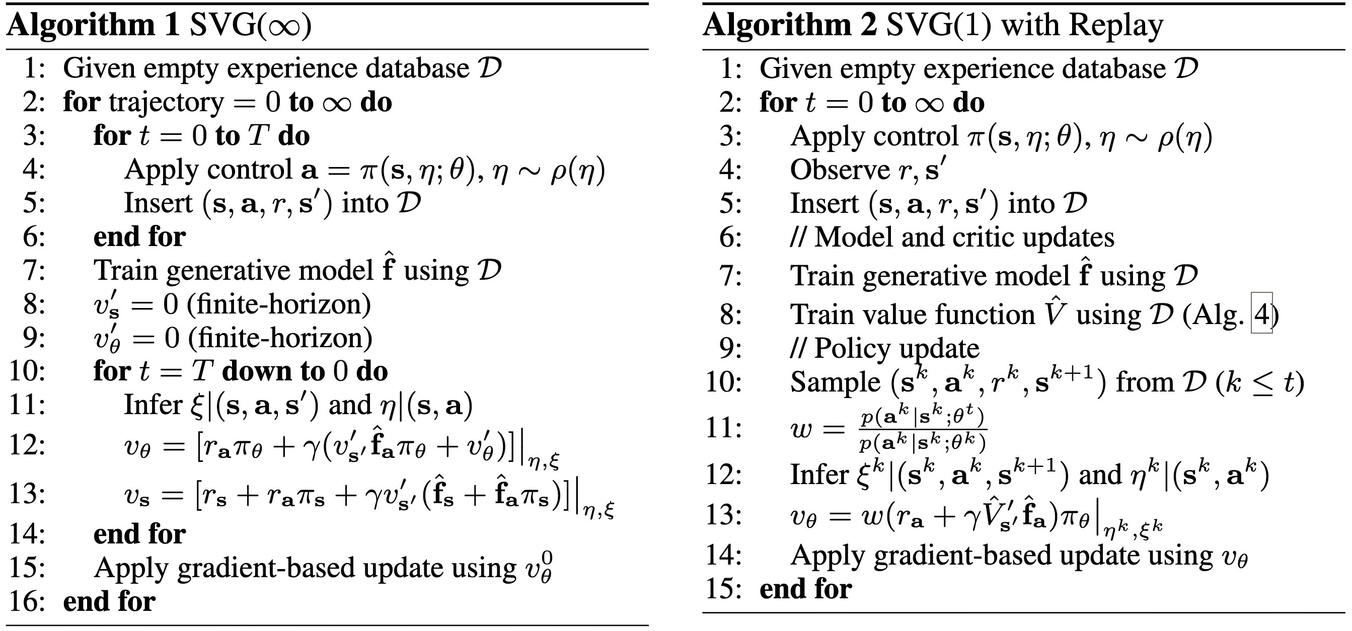
\[\begin{aligned} & v_{\mathbf{s}}=\left.\left[r_{\mathbf{s}}+r_{\mathbf{a}} \pi_{\mathbf{s}}+\gamma v_{\mathbf{s}^{\prime}}^{\prime}\left(\hat{\mathbf{f}}_{\mathbf{s}}+\hat{\mathbf{f}}_{\mathbf{a}} \pi_{\mathbf{s}}\right)\right]\right|_{\eta, \xi} \\ & v_\theta=\left.\left[r_{\mathbf{a}} \pi_\theta+\gamma\left(v_{\mathbf{s}^{\prime}}^{\prime} \hat{\mathbf{f}}_{\mathbf{a}} \pi_\theta+v_\theta^{\prime}\right)\right]\right|_{\eta, \xi} \end{aligned}\]where have written lower-case $v$ to emphasize that the quantities are one-sample estimates, $\hat{\mathbf{f}}$ denotes the learned model, and $\vert_{\mathbf{x}}$ means “evaluated at $\mathbf{x}$” and subscripts are abbreviation for partial differentiation; for example, $V_{\mathbf{s}} = \nabla_{\mathbf{s}} V (\mathbf{s})$. This on-policy algorithm (that is, after each episode, a single gradient-based update is made to the policy, and the policy optimization does not revisit those trajectory data again;) is coined as SVG($\boldsymbol{\infty}$).
The off-policy SVG algorithm, SVG(1), constructs an experience replay buffer with importance sampling to increase data-efficiency. It maintains a database $\mathcal{D}$ with tuples of past state transitions $(\mathbf{s}^k, \mathbf{a}^k, r^k, \mathbf{s}^{k+1})$. At timestep $t$, the importance-weight equals to
\[w \triangleq \frac{p(\mathbf{a}^k \vert \mathbf{s}^k; \theta^t)}{p(\mathbf{a}^k \vert \mathbf{s}^k; \theta^k)}\]where $\theta^k$ is the policy parameters in use at the historical timestep $k$.
Decision-Time Planning
While background planning learns how to act for any situations by optimizing the expected return \(\mathbb{E}_{\mathbf{s}_0 \in \mathcal{S}} [ \sum_{t=0}^T \gamma^t r(\mathbf{s}_t, \mathbf{a}_t)]\) in the background at the learning stage, decision-time planning aims to plan the best sequence of actions $\mathbf{a}_t, \cdots \mathbf{a}_T$ just for the current state $\mathbf{s}_t$, i.e.
\[\mathbf{a}_{t:T} = \underset{\mathbf{a}_{t:T}}{\text{argmax}} \; \mathbb{E}_{\mathbf{s}_{t^\prime+1} \sim f_\phi (\mathbf{s}_{t^\prime}, \mathbf{a}_{t^\prime})} \left[\sum_{t^\prime=t}^T \gamma^{t^\prime} r (\mathbf{s}_{t^\prime}, \mathbf{a}_{t^\prime}) \vert \mathbf{a}_{t:T}\right]\]in decision time. This formulation aligns with the decision-making problems, particularly optimal control problem (thus, the term (optimal) control frequently appears in the MBRL field). The optimal control theory aims to define control variables of a dynamic control system, which minimizes (or maximizes) some performance criterion and at the same time satifies the physical constraints. For example, given the current state $\bar{\mathbf{x}}_t$ and assuming discrete-time formulations, the problem can be mathematically formulated as
\[\begin{aligned} \min _{\mathbf{x}, \mathbf{u}} & \sum_{t^\prime=t}^T c_t \left(\mathbf{x}_{t^\prime}, \mathbf{u}_{t^\prime}\right) \\ \text { s.t. } & \mathbf{x}_{t^\prime}=\bar{\mathbf{x}}_{t^\prime} \\ & \mathbf{x}_{t^\prime+1}=f\left(\mathbf{x}_{t^\prime}, \mathbf{u}_{t^\prime}\right) \quad t^\prime=t, \ldots, T-1 \end{aligned}\]where $f$ is the dynamics of the system, $c_t$, $\mathbf{x}_t$, and $\mathbf{u}_t$ are the cost function (counterpart of negative reward function in RL), the state, and the control (counterpart of action in RL) at timestep $t$, respectively. Hence, the problem of reinforcement learning can be considered as the optimal control of incompletely-known MDPs.
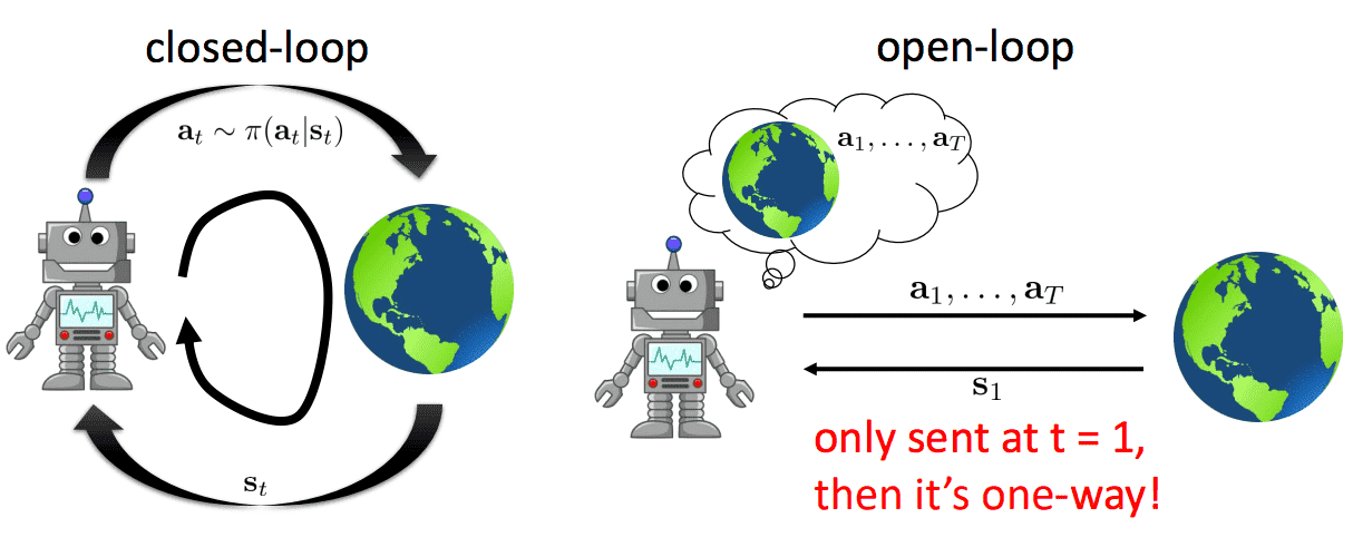
The types of solution to the control problem, or the control problem itself can be categorized into two distinct branches: closed-loop and open-loop frameworks. In an open-loop system plans a sequence of actions aimed at maximizing the expected reward without receiving actual feedback from the environment which resembles the planning. In contrast, a closed-loop system, upon the agent producing an action, feedback is provided as the world is updated, resulting in the observation of the subsequent state. This feedback loop iterates continuously. In this case, $f$ should be the actual dynamics of the environment. (Note that the actual operational flow of RL typically follows a closed-loop structure.)
Although control theory conventionally addressed closed-loop problems, there has been a notable surge in interest toward designing algorithms that find feasible open-loop trajectories for nonlinear systems. And some of this work have been applied the term “motion planning” with a different interpretation from its use in other fields. Thus, even though each originally considered different problems, the fields of robotics, artificial intelligence, and control theory have expanded their scope and use of the term “planning” to share an interesting common ground. Hence, to my knowledge, planning can be used in a broad sense that encompasses this common ground including the optimal control.
Since optimal control solvers generally utilize the derivative, one important distinction between planning methods, especially decision-time planning is whether they require differentiability of the model.
Discrete Planning
Discrete planning is the main approach in the classic AI and RL, where we assume the discrete state-action space and implement discrete back-ups which are stored in a tree, table or used as training targets to improve a value or policy function.
Cross-Entropy Method (CEM)
The cross-entropy method (CEM) selects $N$ action sequences from a distribution (e.g. Gaussian), then cherry-picks the top $M < N$ “elite” actions sequences, ordered by the highest return, and then refits the initial distribution of the action sequences to be more similar to the elites.
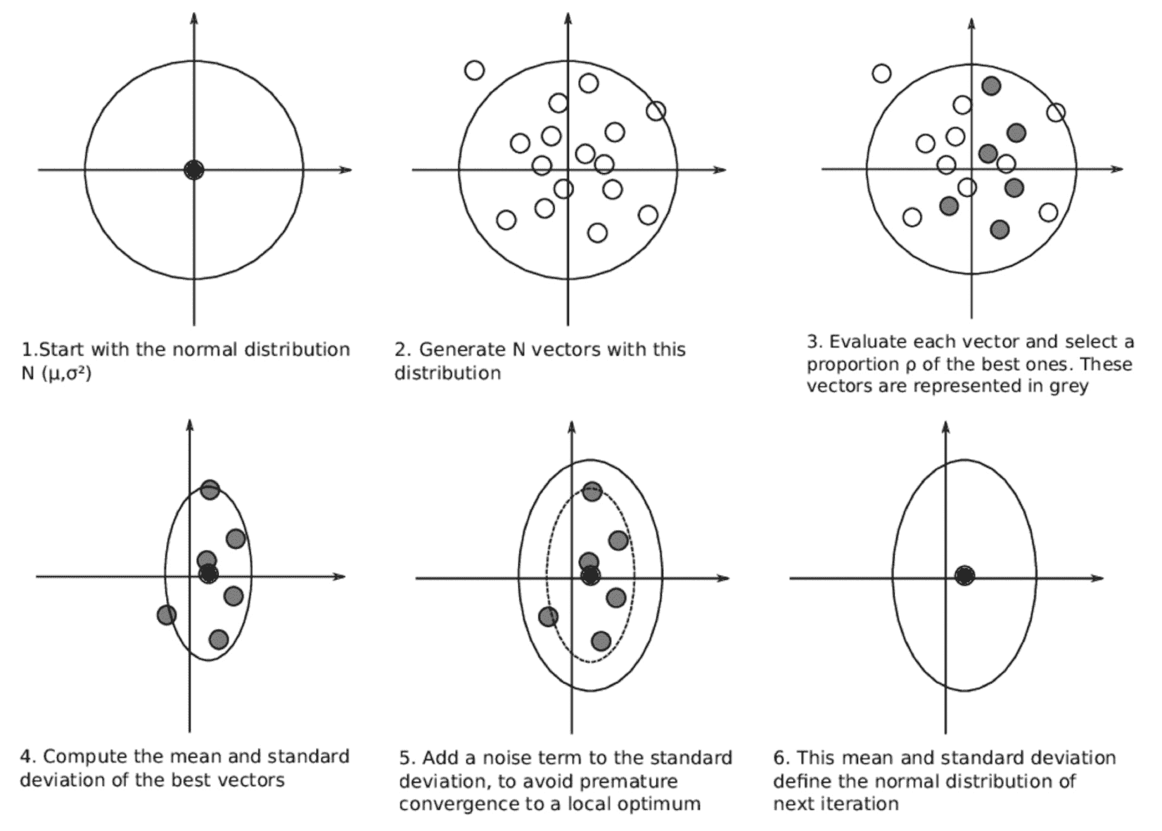
This planning method is simple to implement and fast because it can be parallelized to execute independent trajectories. However, it is limited to lower dimension problems and can only be used in the open-loop style of planning.
Monte-Carlo Tree Search (MCTS)
Rollout algorithms are decision-time planning algorithms based on Monte-Carlo control applied to simulated trajectories that all begin at the current environment state. They estimate action values for a given policy (called rollout policy) by averaging the returns of many simulated trajectories that start with each possible action and then follow the given policy. When the action-value estimates are considered to be accurate enough, the action (or one of the actions) having the highest estimated value is executed, after which the process is carried out anew from the resulting next state.
Monte-Carlo Tree Search (MCTS) stands out as a remarkably successful instance of decision-time planning that is a type of rollout algorithm at its base. MCTS is further enhanced by leveraging knowledge from previous simulation; the addition of means for accumulating value estimates obtained from the Monte Carlo simulations, thereby guiding subsequent simulations towards trajectories that promise higher rewards. MCTS has demonstrated its effectiveness across diverse competitive domains, and its fame soared notably through its implementation in AlphaGo and subsequent successes.
MCTS requires two sort of policies for simulation:
- Tree policy, which is based on the estimated $Q(\mathbf{s}, \mathbf{a})$ that improves during search; exploiting the knowledge from prior steps
- Rollout policy, which is fixed that we use to get the monte Carlo estimate of the return from the leaf onward
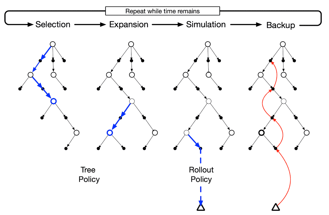
Then it just repreats the following four steps for each simulated episode until the programmer have exhausted the computational time or computational resources allocated to the action selection.
- Selection
Starting at the root node, i.e. the current state $\mathbf{s}_t$ the tree policy, based on the current estimate of $Q (\mathbf{s}, \mathbf{a})$, traverses until it reaches a leaf node. - Expansion
On some iterations (depending on details of the application), the tree is expanded from the selected leaf node by adding one or more child nodes reached from the selected node via unexplored actions. - Simulation
From the selected node, or from one of its newly-added child nodes (if any), $K$ simulation of a complete episode is run with actions selected by the rollout policy. Consequently, it obtains Monte-Carlo trial $$ \{ \mathbf{s}_t, \mathbf{a}_t^k, r_{t}^k, \mathbf{s}_{t+1}^k, \mathbf{a}_{t+1}^k, \cdots, r_{T-1}^k, \mathbf{s}_T^k \}_{k=1}^K \sim \pi_{\textrm{rollout}} $$ - Backup
Update $Q(\mathbf{s}, \mathbf{a})$ backward for all state-action pairs $(\mathbf{s}, \mathbf{a})$ in the tree with the following update rule: $$ Q(\mathbf{s}, \mathbf{a}) = \frac{1}{N(\mathbf{s}, \mathbf{a})} \sum_{k=1}^K \sum_{t^\prime = t}^T \boldsymbol{1} (\mathbf{s}_{t^\prime}^k = \mathbf{s}, \mathbf{a}_{t^\prime}^k = \mathbf{a}) \cdot G_{t^\prime}^k $$ where $N(\mathbf{s}, \mathbf{a})$ stores the number of visits.
Several methods can be used to implement both the tree and rollout policies. A popular implementation for the tree policy is the selection rule employed by the upper confidence bounds (UCB) applied to trees (called UCT) algorithm, which is defined as
\[\mathbf{a}^* = \underset{\mathbf{a} \in \mathcal{A}}{\text{argmax}} \left\{ Q (\mathbf{s}, \mathbf{a}) + C \sqrt{\frac{\ln N(\mathbf{s})}{N (\mathbf{s}, \mathbf{a})}}\right\}\]where $C$ is an exploration constant used to balance exploration and exploitation. Observe that the large $C$ encourages the exploration of less-visited action choices. And the rollout policy is commonly implemented via a uniform random selection policy.
Optimal Control & Trajectory Optimization
If we relieve the discrete constraint for state-action space, it is possible to derive the derivatives such as $\frac{\mathrm{d}f}{\mathrm{d} \mathbf{x}_t}$ and $\frac{\mathrm{d}f}{\mathrm{d} \mathbf{u}_t}$. In such scenarios, trajectory optimization can be employed as decision-time planning algorithm. Trajectory optimization methods are considered as a subset of the more general field of optimal control. They generally re-formulate the optimal control problem as a finite-dimensional optimization problem (e.g. discretize the continuous-time trajectory, etc.) over some representation of the state and control trajectory, and then solving the optimization problem usually using a gradient-based technique.
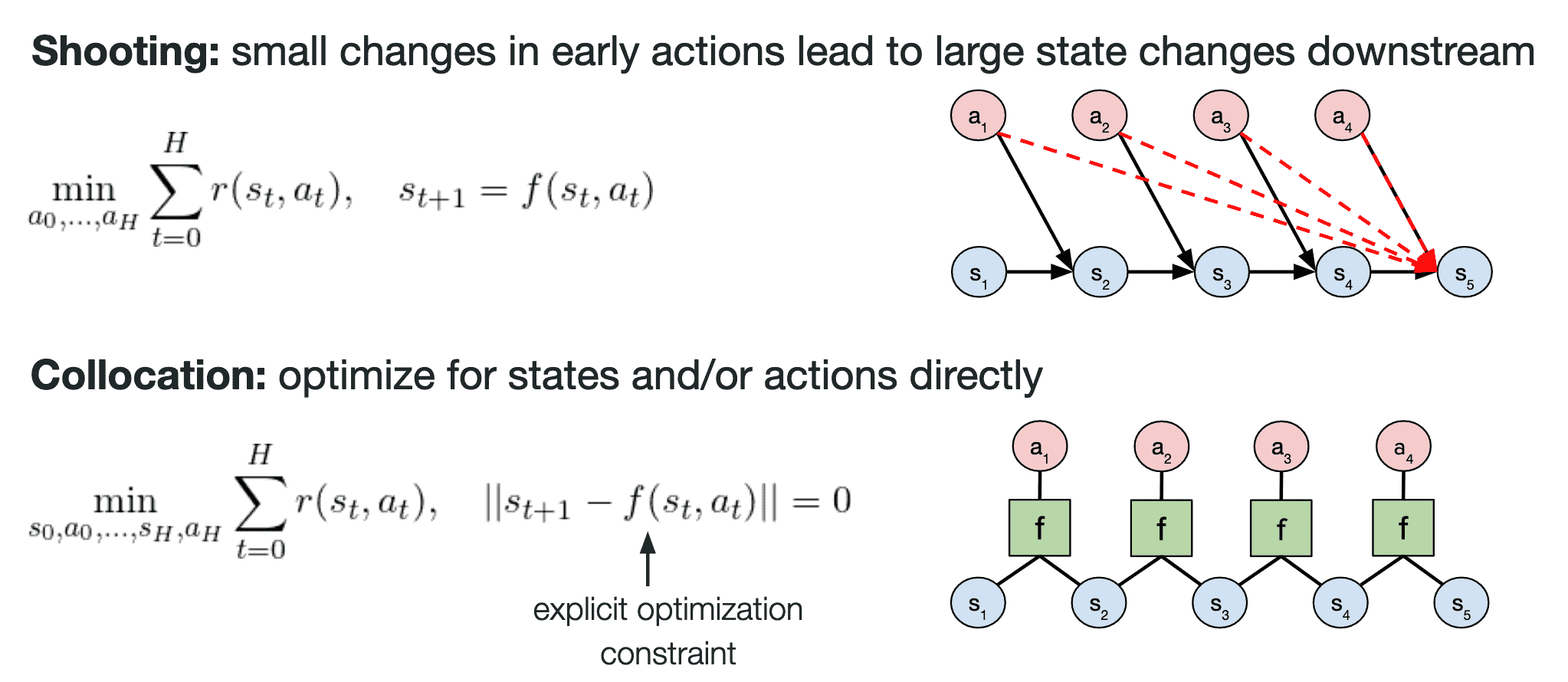
Theoretically, trajectory optimization methodologies can be categorized into shooting methods and collocation methods, based on whether they treat states as trainable parameters. This post will concentrate on shooting methods.
Linear Quadratic Regulator (LQR)
In its simplest form, the Linear quadratic regulator (LQR) shows that the optimal control $\mathbf{u}_t$ has a closed-form solution that depends on $\mathbf{x}_t$ under certain simplifying assumptions. Specifically, optimal $\mathbf{u}_t$ is linear in $\mathbf{x}_t$ for every timestep, assuming the linear dynamics $f$ and quadratic costs $c$ in the states $\mathbf{x}_t$ and controls $\mathbf{u}_t$:
\[\begin{aligned} f\left(\mathbf{x}_t, \mathbf{u}_t\right) & = \mathbf{F}_t\left[\begin{array}{l} \mathbf{x}_t \\ \mathbf{u}_t \end{array}\right]+ \mathbf{f}_t \\ c(\mathbf{x}_t, \mathbf{u}_t) & = \frac{1}{2} \left[\begin{array}{l} \mathbf{x}_t \\ \mathbf{u}_t \end{array}\right]^\top \mathbf{C}_t \left[\begin{array}{l} \mathbf{x}_t \\ \mathbf{u}_t \end{array}\right] + \left[\begin{array}{l} \mathbf{x}_t \\ \mathbf{u}_t \end{array}\right]^\top \mathbf{c}_t \end{aligned}\]We define the quantity $Q(\mathbf{x}_t, \mathbf{u}_t)$ to be the cost-to-go; the sum of the remaining costs from time $t$ to $T$:
\[Q(\mathbf{x}_t, \mathbf{u}_t) = \sum_{t^\prime = t}^T c(\mathbf{x}_{t^\prime}, \mathbf{u}_{t^\prime}) \text{ s.t. } \mathbf{x}_{t^\prime} = f (\mathbf{x}_{t^\prime - 1}, \mathbf{u}_{t^\prime-1} )\]and define the value function $V (\mathbf{x}_t)$ as
\[V(\mathbf{x}_t) = \underset{\mathbf{u}_t}{\min} Q (\mathbf{x}_t, \mathbf{u}_t)\]Then, we can obtain the following recursive relations:
- As a base case, $\mathbf{u}_T$ that minimizes $Q(\mathbf{x}_t, \mathbf{u}_T)$ is linear in $\mathbf{x}_T$: $$ \mathbf{u}_T^* = \underset{\mathbf{u}_T}{\text{argmin}} \; Q(\mathbf{x}_T, \mathbf{u}_T) = \mathbf{K}_T \mathbf{x}_T + \mathbf{k}_T $$ Moreover, $V(\mathbf{x}_T)$ is quadratic in $\mathbf{x}_T$: $$ V(\mathbf{x}_T) = \frac{1}{2} \mathbf{x}_T^\top \mathbf{V}_T \mathbf{x}_T + \mathbf{x}_T^\top \mathbf{v}_T $$
- $Q(\mathbf{x}_{T-1}, \mathbf{u}_{T-1})$ is quadratic in $\mathbf{x}_T$ and $\mathbf{u}_T$: $$ Q(\mathbf{x}_{T-1}, \mathbf{u}_{T-1}) = \frac{1}{2} \left[\begin{array}{l} \mathbf{x}_{T-1} \\ \mathbf{u}_{T-1} \end{array}\right]^\top \mathbf{Q}_{T-1} \left[\begin{array}{l} \mathbf{x}_{T-1} \\ \mathbf{u}_{T-1} \end{array}\right] + \left[\begin{array}{l} \mathbf{x}_{T-1} \\ \mathbf{u}_{T-1} \end{array}\right]^\top \mathbf{q}_{T-1} $$ And $\mathbf{u}_{T-1}$ that minimizes $Q(\mathbf{x}_{T-1}, \mathbf{u}_{T-1})$ is again linear in $\mathbf{x}_{T-1}$: $$ \mathbf{u}_{T-1}^* = \underset{\mathbf{u}_{T-1}}{\text{argmin}} \; Q(\mathbf{x}_{T-1}, \mathbf{u}_{T-1}) = \mathbf{K}_{T-1} \mathbf{x}_{T-1} + \mathbf{k}_{T-1} $$
$\color{red}{\mathbf{Proof.}}$
For base case, we solve for $\mathbf{u}_T$ first. Let
\[\begin{aligned} & \mathbf{C}_T=\left[\begin{array}{ll} \mathbf{C}_{\mathbf{x}_T, \mathbf{x}_T} & \mathbf{C}_{\mathbf{x}_T, \mathbf{u}_T} \\ \mathbf{C}_{\mathbf{u}_T, \mathbf{x}_T} & \mathbf{C}_{\mathbf{u}_T, \mathbf{u}_T} \end{array}\right] \\ & \mathbf{c}_T=\left[\begin{array}{l} \mathbf{c}_{\mathbf{x}_T} \\ \mathbf{c}_{\mathbf{u}_T} \end{array}\right] \end{aligned}\]Then, the gradient of $Q (\mathbf{x}_T, \mathbf{u}_T)$ is given by
\[\nabla_{\mathbf{u}_T} Q (\mathbf{x}_T, \mathbf{u}_T) = \mathbf{C}_{\mathbf{u}_T, \mathbf{x}_T} \mathbf{x}_T + \mathbf{C}_{\mathbf{u}_T, \mathbf{u}_T} \mathbf{u}_T + \mathbf{c}_{\mathbf{u}_T}^\top\]Setting $\nabla_{\mathbf{u}_T} Q (\mathbf{x}_T, \mathbf{u}_T) = 0$, we obtain the optimal control:
\[\begin{aligned} \mathbf{u}_T^* & = - \mathbf{C}_{\mathbf{u}_T, \mathbf{u}_T}^{-1} (\mathbf{C}_{\mathbf{u}_T, \mathbf{x}_T} \mathbf{x}_T + \mathbf{c}_{\mathbf{u}_T}) \\ & = \mathbf{K}_T \mathbf{x}_T + \mathbf{k}_T \end{aligned}\]where
\[\begin{aligned} \mathbf{K}_T & = - \mathbf{C}_{\mathbf{u}_T, \mathbf{u}_T}^{-1} \mathbf{C}_{\mathbf{u}_T, \mathbf{x}_T} \\ \mathbf{k}_T & = - \mathbf{C}_{\mathbf{u}_T, \mathbf{u}_T}^{-1} \mathbf{c}_{\mathbf{u}_T} \end{aligned}\]Since $\mathbf{u}_T$ is fully determined by $\mathbf{x}_T$, we can obtain the value $V(\mathbf{x}_T)$ by eliminating $\mathbf{u}_T$ via substitution:
\[\begin{aligned} V\left(\mathbf{x}_T\right)= & \; \frac{1}{2}\left[\begin{array}{c} \mathbf{x}_T \\ \mathbf{K}_T \mathbf{x}_T+\mathbf{k}_T \end{array}\right]^\top \mathbf{C}_T\left[\begin{array}{c} \mathbf{x}_T \\ \mathbf{K}_T \mathbf{x}_T+\mathbf{k}_T \end{array}\right]+\left[\begin{array}{c} \mathbf{x}_T \\ \mathbf{K}_T \mathbf{x}_T+\mathbf{k}_T \end{array}\right]^\top \mathbf{c}_T \\ = & \; \frac{1}{2} \mathbf{x}_T^\top \mathbf{C}_{\mathbf{x}_T, \mathbf{x}_T} \mathbf{x}_T+\frac{1}{2} \mathbf{x}_T^\top \mathbf{C}_{\mathbf{x}_T, \mathbf{u}_T} \mathbf{K}_T \mathbf{x}_T+\frac{1}{2} \mathbf{x}_T^\top \mathbf{K}_T^\top \mathbf{C}_{\mathbf{u}_T, \mathbf{x}_T} \mathbf{x}_T+\frac{1}{2} \mathbf{x}_T^\top \mathbf{K}_T^\top \mathbf{C}_{\mathbf{u}_T, \mathbf{u}_T} \mathbf{K}_T \mathbf{x}_T \\ & + \mathbf{x}_T^\top \mathbf{K}_T^\top \mathbf{C}_{\mathbf{u}_T, \mathbf{u}_T} \mathbf{k}_T+\frac{1}{2} \mathbf{x}_T^\top \mathbf{C}_{\mathbf{x}_T, \mathbf{u}_T} \mathbf{k}_T+\mathbf{x}_T^\top \mathbf{c}_{\mathbf{x}_T}+\mathbf{x}_T^\top \mathbf{K}_T^\top \mathbf{c}_{\mathbf{u}_T} \\ = & \; \frac{1}{2} \mathbf{x}_T^\top \mathbf{V}_T \mathbf{x}_T+\mathbf{x}_T^\top \mathbf{v}_T \end{aligned}\]where
\[\begin{aligned} \mathbf{V}_T & = \mathbf{C}_{\mathbf{x}_T, \mathbf{x}_T} + \mathbf{C}_{\mathbf{x}_T, \mathbf{u}_T} \mathbf{K}_T + \mathbf{K}_T^\top \mathbf{C}_{\mathbf{u}_T, \mathbf{x}_T} + \mathbf{K}_T^\top \mathbf{C}_{\mathbf{u}_T, \mathbf{u}_T} \mathbf{K}_T \\ \mathbf{v}_T & = \mathbf{c}_{\mathbf{x}_T} + \mathbf{C}_{\mathbf{x}_T, \mathbf{u}_T} \mathbf{k}_T + \mathbf{K}_T^\top \mathbf{c}_{\mathbf{u}_T} + \mathbf{K}_T^\top \mathbf{C}_{\mathbf{u}_T, \mathbf{u}_T} \mathbf{k}_T \end{aligned}\]From \(\mathbf{x}_T = f(\mathbf{x}_{T-1}, \mathbf{u}_{T-1}) = \mathbf{x}_T = \mathbf{F}_{T-1} \left[\begin{array}{c} \mathbf{x}_{T-1} \\ \mathbf{u}_{T-1} \end{array}\right] + \mathbf{f}_{T-1}\), $V(\mathbf{x}_T)$ is re-written as
\[V(\mathbf{x}_T) = \frac{1}{2} \left[\begin{array}{c} \mathbf{x}_{T-1} \\ \mathbf{u}_{T-1} \end{array}\right]^\top \mathbf{F}_{T-1}^\top \mathbf{V}_T \mathbf{F}_{T-1} \left[\begin{array}{c} \mathbf{x}_{T-1} \\ \mathbf{u}_{T-1} \end{array}\right] + \left[\begin{array}{c} \mathbf{x}_{T-1} \\ \mathbf{u}_{T-1} \end{array}\right]^\top \mathbf{F}_{T-1}^\top \mathbf{V}_T \mathbf{f}_{T-1} + \left[\begin{array}{c} \mathbf{x}_{T-1} \\ \mathbf{u}_{T-1} \end{array}\right]^\top \mathbf{F}_{T-1}^\top \mathbf{v}_T\]By selecting \(\mathbf{u}_T = \mathbf{u}_T^*\) at timestep $t = T$, we may write \(Q(\mathbf{x}_{T-1}, \mathbf{u}_{T-1}) = \mathbf{c}(\mathbf{x}_{T-1}, \mathbf{u}_{T-1}) + V(\mathbf{x}_T)\). That is, \(Q(\mathbf{x}_{T-1}, \mathbf{u}_{T-1})\) is again quadratic:
\[Q(\mathbf{x}_{T-1}, \mathbf{u}_{T-1}) = \frac{1}{2} \left[\begin{array}{l} \mathbf{x}_{T-1} \\ \mathbf{u}_{T-1} \end{array}\right]^\top \mathbf{Q}_{T-1} \left[\begin{array}{l} \mathbf{x}_{T-1} \\ \mathbf{u}_{T-1} \end{array}\right] + \left[\begin{array}{l} \mathbf{x}_{T-1} \\ \mathbf{u}_{T-1} \end{array}\right]^\top \mathbf{q}_{T-1}\]where
\[\begin{aligned} \mathbf{Q}_{T-1} & = \mathbf{C}_{T-1} + \mathbf{F}_{T-1}^\top \mathbf{V}_T \mathbf{F}_{T-1} \\ \mathbf{q}_{T-1} & = \mathbf{c}_{T-1} + \mathbf{F}_{T-1}^\top \mathbf{V}_T \mathbf{f}_{T-1} + \mathbf{F}_{T-1}^\top \mathbf{v}_T \end{aligned}\]Then, the gradient of \(Q (\mathbf{x}_{T-1}, \mathbf{u}_{T-1})\) is given by
\[\nabla_{\mathbf{u}_{T-1}} Q (\mathbf{x}_{T-1}, \mathbf{u}_{T-1}) = \mathbf{Q}_{\mathbf{u}_{T-1}, \mathbf{x}_{T-1}} \mathbf{x}_{T-1} + \mathbf{Q}_{\mathbf{u}_{T-1}, \mathbf{u}_{T-1}} \mathbf{u}_{T-1} + \mathbf{q}_{\mathbf{u}_{T-1}}^\top\]Setting \(\nabla_{\mathbf{u}_{T-1}} Q (\mathbf{x}_{T-1}, \mathbf{u}_{T-1}) = 0\), we obtain
\[\mathbf{u}_{T-1}^* = \mathbf{K}_{T-1} \mathbf{x}_{T-1} + \mathbf{k}_{T-1}\]where
\[\begin{aligned} \mathbf{K}_{T-1} & = - \mathbf{Q}_{\mathbf{u}_{T-1}, \mathbf{u}_{T-1}} \mathbf{Q}_{\mathbf{u}_{T-1}, \mathbf{x}_{T-1}} \\ \mathbf{k}_{T-1} & = - \mathbf{Q}_{\mathbf{u}_{T-1}, \mathbf{u}_{T-1}} \mathbf{q}_{\mathbf{u}_{T-1}} \end{aligned}\] \[\tag*{$\blacksquare$}\]The above theorem furnishes us with the pseudocode:
\[\begin{aligned} & \text{for } t=T \text{ to } 1 \\ & \quad \mathbf{Q}_t=\mathbf{C}_t+\mathbf{F}_t^T \mathbf{V}_{t+1} \mathbf{F}_t, \; \mathbf{q}_t=\mathbf{c}_t+\mathbf{F}_t^T \mathbf{V}_{t+1} \mathbf{f}_t+\mathbf{F}_t^T \mathbf{v}_{t+1} \\ & \quad Q\left(\mathbf{x}_t, \mathbf{u}_t\right)=\operatorname{const}+\frac{1}{2}\left[\begin{array}{c} \mathbf{x}_t \\ \mathbf{u}_t \end{array}\right]^T \mathbf{Q}_t\left[\begin{array}{c} \mathbf{x}_t \\ \mathbf{u}_t \end{array}\right]+\left[\begin{array}{c} \mathbf{x}_t \\ \mathbf{u}_t \end{array}\right]^T \mathbf{q}_t \\ & \quad \mathbf{u}_t \leftarrow \arg \min _{\mathbf{u}_t} Q\left(\mathbf{x}_t, \mathbf{u}_t\right)=\mathbf{K}_t \mathbf{x}_t+\mathbf{k}_t \\ & \quad \mathbf{K}_t=-\mathbf{Q}_{\mathbf{u}_t, \mathbf{u}_t}^{-1} \mathbf{Q}_{\mathbf{u}_t, \mathbf{x}_t}, \; \mathbf{k}_t=-\mathbf{Q}_{\mathbf{u}_t, \mathbf{u}_t}^{-1} \mathbf{q}_{\mathbf{u}_t} \\ & \quad \mathbf{V}_t=\mathbf{Q}_{\mathbf{x}_t, \mathbf{x}_t}+\mathbf{Q}_{\mathbf{x}_t, \mathbf{u}_t} \mathbf{K}_t+\mathbf{K}_t^T \mathbf{Q}_{\mathbf{u}_t, \mathbf{x}_t}+\mathbf{K}_t^T \mathbf{Q}_{\mathbf{u}_t, \mathbf{u}_t} \mathbf{K}_t \\ & \quad \mathbf{v}_t=\mathbf{q}_{\mathbf{x}_t}+\mathbf{Q}_{\mathbf{x}_t, \mathbf{u}_t} \mathbf{k}_t+\mathbf{K}_t^T \mathbf{Q}_{\mathbf{u}_t}+\mathbf{K}_t^T \mathbf{Q}_{\mathbf{u}_t, \mathbf{u}_t} \mathbf{k}_t \\ & \quad V\left(\mathbf{x}_t\right)=\operatorname{const}+\frac{1}{2} \mathbf{x}_t^T \mathbf{V}_t \mathbf{x}_t+\mathbf{x}_t^T \mathbf{v}_t \\ & \text{for } t=1 \text{ to } T \\ & \quad \mathbf{u}_t=\mathbf{K}_t \mathbf{x}_t + \mathbf{k}_t \\ & \quad \mathbf{x}_{t+1} = f(\mathbf{x}_t, \mathbf{u}_t) \\ \end{aligned}\]iterative LQR (iLQR)
In the non-linear system, we can approximate the dynamic model as linear to the first order and the cost function as quadratic to the second order:
\[\begin{aligned} f\left(\mathbf{x}_t, \mathbf{u}_t\right) & \approx f\left(\hat{\mathbf{x}}_t, \hat{\mathbf{u}}_t\right)+\nabla_{\mathbf{x}_t, \mathbf{u}_t} f\left(\hat{\mathbf{x}}_t, \hat{\mathbf{u}}_t\right)\left[\begin{array}{l} \mathbf{x}_t-\hat{\mathbf{x}}_t \\ \mathbf{u}_t-\hat{\mathbf{u}}_t \end{array}\right] \\ c\left(\mathbf{x}_t, \mathbf{u}_t\right) & \approx c\left(\hat{\mathbf{x}}_t, \hat{\mathbf{u}}_t\right)+\nabla_{\mathbf{x}_t, \mathbf{u}_t} c\left(\hat{\mathbf{x}}_t, \hat{\mathbf{u}}_t\right)^\top \left[\begin{array}{l} \mathbf{x}_t-\hat{\mathbf{x}}_t \\ \mathbf{u}_t-\hat{\mathbf{u}}_t \end{array}\right]+\frac{1}{2}\left[\begin{array}{l} \mathbf{x}_t-\hat{\mathbf{x}}_t \\ \mathbf{u}_t-\hat{\mathbf{u}}_t \end{array}\right]^T \nabla_{\mathbf{x}_t, \mathbf{u}_t}^2 c\left(\hat{\mathbf{x}}_t, \hat{\mathbf{u}}_t\right)\left[\begin{array}{l} \mathbf{x}_t-\hat{\mathbf{x}}_t \\ \mathbf{u}_t-\hat{\mathbf{u}}_t \end{array}\right] \end{aligned}\]By rearranging the terms, we can reformulate the equations as:
\[\begin{gathered} \begin{aligned} f\left(\mathbf{x}_t, \mathbf{u}_t\right) - f\left(\hat{\mathbf{x}}_t, \hat{\mathbf{u}}_t\right) & = \nabla_{\mathbf{x}_t, \mathbf{u}_t} f\left(\hat{\mathbf{x}}_t, \hat{\mathbf{u}}_t\right)\left[\begin{array}{l} \mathbf{x}_t-\hat{\mathbf{x}}_t \\ \mathbf{u}_t-\hat{\mathbf{u}}_t \end{array}\right] \\ c\left(\mathbf{x}_t, \mathbf{u}_t\right) - c\left(\hat{\mathbf{x}}_t, \hat{\mathbf{u}}_t\right) & = \frac{1}{2}\left[\begin{array}{l} \mathbf{x}_t-\hat{\mathbf{x}}_t \\ \mathbf{u}_t-\hat{\mathbf{u}}_t \end{array}\right]^\top \nabla_{\mathbf{x}_t, \mathbf{u}_t}^2 c\left(\hat{\mathbf{x}}_t, \hat{\mathbf{u}}_t\right)\left[\begin{array}{l} \mathbf{x}_t-\hat{\mathbf{x}}_t \\ \mathbf{u}_t-\hat{\mathbf{u}}_t \end{array}\right] + \left[\begin{array}{l} \mathbf{x}_t-\hat{\mathbf{x}}_t \\ \mathbf{u}_t-\hat{\mathbf{u}}_t \end{array}\right]^\top \nabla_{\mathbf{x}_t, \mathbf{u}_t} c\left(\hat{\mathbf{x}}_t, \hat{\mathbf{u}}_t\right) \end{aligned} \\ \Downarrow \\ \begin{aligned} \bar{f} \left(\delta\mathbf{x}_t, \delta\mathbf{u}_t\right) & = \underbrace{\mathbf{F}_T}_{\nabla_{\mathbf{x}_t, \mathbf{u}_t} f\left(\hat{\mathbf{x}}_t, \hat{\mathbf{u}}_t\right)} \left[\begin{array}{l} \delta \mathbf{x}_t \\ \delta \mathbf{u}_t \end{array}\right] \\ \bar{c}\left(\delta\mathbf{x}_t, \delta\mathbf{u}_t\right) & = \frac{1}{2}\left[\begin{array}{l} \mathbf{x}_t-\hat{\mathbf{x}}_t \\ \mathbf{u}_t-\hat{\mathbf{u}}_t \end{array}\right]^\top \underbrace{\mathbf{C}_t}_{\nabla_{\mathbf{x}_t, \mathbf{u}_t}^2 c\left(\hat{\mathbf{x}}_t, \hat{\mathbf{u}}_t\right)}\left[\begin{array}{l} \delta\mathbf{x}_t \\ \delta\mathbf{u}_t \end{array}\right] + \left[\begin{array}{l} \delta\mathbf{x}_t \\ \delta\mathbf{u}_t \end{array}\right]^\top \underbrace{\mathbf{c}_t}_{\nabla_{\mathbf{x}_t, \mathbf{u}_t} c\left(\hat{\mathbf{x}}_t, \hat{\mathbf{u}}_t\right)} \end{aligned} \end{gathered}\]where $\delta \mathbf{x}_t = \mathbf{x}_T - \hat{\mathbf{x}}_t$ and $\delta \mathbf{u}_t = \mathbf{u}_T - \hat{\mathbf{u}}_t$. LQR can then be applied to the approximated model $\bar{f}$, cost $\bar{c}$, state $\delta \mathbf{x}_t$, and action $\delta \mathbf{u}_t$. This is known as iterative LQR (iLQR).
In fact, iLQR is an approximation of Newton’s method, which iteratively update its solution by approximating with Taylor expansion for computing $\min_{\mathbf{x}} g(\mathbf{x})$:
\[\begin{aligned} \mathbf{g} & = \nabla_{\mathbf{x}} g(\hat{\mathbf{x}}) \\ \mathbf{H} & = \nabla_{\mathbf{x}}^2 g(\hat{\mathbf{x}}) \\ \hat{\mathbf{x}} & \leftarrow \underset{\mathbf{x}}{\text{argmin}} \; \frac{1}{2} (\mathbf{x} - \hat{\mathbf{x}})^\top \mathbf{H} (\mathbf{x} - \hat{\mathbf{x}}) + \mathbf{g}^\top (\mathbf{x} - \hat{\mathbf{x}}) \end{aligned}\]Differential Dynamic Programming (DDP)
The iLQR method does not expand the dynamics to the second order, thus it is an approximation of Newton’s method. To get Newton’s method, it requires the second order dynamics approximation:
\[f\left(\mathbf{x}_t, \mathbf{u}_t\right) \approx f\left(\hat{\mathbf{x}}_t, \hat{\mathbf{u}}_t\right)+\nabla_{\mathbf{x}_t, \mathbf{u}_t} f\left(\hat{\mathbf{x}}_t, \hat{\mathbf{u}}_t\right)\left[\begin{array}{l} \delta\mathbf{x}_t \\ \delta\mathbf{u}_t \end{array}\right] + \frac{1}{2} \left[\begin{array}{l} \delta\mathbf{x}_t \\ \delta\mathbf{u}_t \end{array}\right]^\top \nabla_{\mathbf{x}_t, \mathbf{u}_t}^2 f(\hat{\mathbf{x}}_t, \hat{\mathbf{u}}_t) \left[\begin{array}{l} \delta\mathbf{x}_t \\ \delta\mathbf{u}_t \end{array}\right]\]and it is termed differential dynamic programming (DDP).
References
[1] Reinforcement Learning: An Introduction. Richard S. Sutton and Andrew G. Barto, The MIT Press.
[2] Introduction to Reinforcement Learning with David Silver
[3] Foundations of Reinforcement Learning with Applications in Finance by Ashwin Rao
[4] Dyna-Q Algorithm Reinforcement Learning
[5] Feinberg et al. “Model-Based Value Estimation for Efficient Model-Free Reinforcement Learning”. arXiv:1803.00101
[6] Buckman et al. “Sample-Efficient Reinforcement Learning with Stochastic Ensemble Value Expansion”. arXiv:1807.01675
[7] Kurutach et al. “Model-Ensemble Trust-Region Policy Optimization”. arXiv:1802.10592.
[8] Hesse et al. “Learning Continuous Control Policies by Stochastic Value Gradients”. NIPS 2015.
[9] Kris Hauser, “Robotic Systems”
[10] Steven M. LaValle, “Planning Algorithms”, Cambridge University Press, 842 pages, 2006
[11] Luo et al., “A Survey on Model-based Reinforcement Learning”, arXiv:2206.09328
[12] Moerland et al., “Model-based Reinforcement Learning: A Survey”, arXiv:2006.16712
[13] “Tutorial on Model-Based Methods in Reinforcement Learning” by Igor Mordatch and Jessica Hamrick, ICML 2020
[14] Donald E. Kirk, “Optimal Control Theory, an Introduction”
Leave a comment