
[RL] Model-Based RL from Pixels
For high-dimensional state spaces, especially image-based domains, representation learning that learns informative latent state or action representation proves invaluable for the environment model building, as it enhances the effectiveness and efficiency. This post concentrates on such model-based approaches, especially RSSM-based methods: PlaNet and the Dreamer family, to solve complex RL tasks with contact dynamics, partial observability, and sparse rewards using only pixel observations.
Since individual image observations generally do not reveal the full state of the environment, we consider a partially observable MDP (POMDP) differentiating (image) observation $\mathbf{o}_t$ and hidden state $\mathbf{s}_t$:
\[\begin{aligned}[t] & \text{Transition function:} && \mathbf{s}_t \sim \mathrm{p}( \mathbf{s}_t \vert \mathbf{s}_{t-1}, \mathbf{a}_{t - 1} ) \\ & \text{Observation function:} && \mathbf{o}_t \sim \mathrm{p}( \mathbf{o}_t \vert \mathbf{s}_{t} ) \\ & \text{Reward function:} && r_t \sim \mathrm{p}( \mathbf{r}_t \vert \mathbf{s}_{t} ) \\ & \text{Policy:} && \mathbf{a}_t \sim \mathrm{p}( \mathbf{a}_t \vert \mathbf{o}_{\leq t}, \mathbf{a}_{< t} ) \\ \end{aligned}\]And our goal is to find a policy \(\mathrm{p}( \mathbf{a}_t \vert \mathbf{o}_{\leq t}, \mathbf{a}_{< t} )\) that maximizes the expected sum of rewards \(\mathbb{E}[\sum_{t=1}^T r_t]\). To infer an approximate hidden latent state from the history, RSSM-based methods learn the representation model \(\mathrm{q}(\mathbf{s}_t \vert \mathbf{h}_{t}, \mathbf{a}_t)\) with recurrent state-space model (RSSM) that stores the history information $\mathbf{h}_t$.
Preliminary: Recurrent State-Space Model (RSSM)
To predict forward in latent state space, PlaNet and the Dreamer family employs recurrent state-space model (RSSM) with sequence VAE that uses the representation model \(\mathrm{q}_{\phi} (\mathbf{s}_t \vert \mathbf{o}_{\leq t})\) as an encoder that compresses visual observation into Markovian hidden state, and decoder \(\mathrm{p}_{\theta} (\mathbf{o}_t \vert \mathbf{s}_t)\).
In generative process, from the latent space of $\mathbf{s}$, the decoder aims to generate the sequence of observation $\mathbf{o}$, following the density:
\[\mathrm{p} (\mathbf{o}_{1:T}, \mathbf{s}_{1:T}) = \prod_{t=1}^T \mathrm{p}_{\theta} (\mathbf{o}_t \vert \mathbf{s}_t ) \mathrm{p}_{\theta} (\mathbf{s}_{t} \vert \mathbf{s}_{t-1})\]where using the transition model \(\mathrm{p}_{\theta}\) as a prior and \(\mathrm{p}_{\theta} (\mathbf{s}_{1} \vert \mathbf{s}_{0}) = \mathrm{p}_{\theta} (\mathbf{s}_{0})\). (Although the parameters of these models are denoted as $\theta$, it’s essential to clarify that they are distinct neural networks.) And to maximize the ELBO, recall that we approximate the intractable true posterior with decoder \(\mathrm{q}_{\phi} (\mathbf{o}_t \vert \mathbf{s}_{\leq t})\) (variational approximation)
\[\mathrm{p}(\mathbf{s}_{1:T} \vert \mathbf{o}_{1:T}) \approx \mathrm{q}_\phi (\mathbf{s}_{1:T} \vert \mathbf{o}_{1:T}) = \prod_{t=1}^T \mathrm{q}_\phi (\mathbf{s}_t \vert \mathbf{o}_{\leq t})\]Then, for maximizing likelihood of sequence VAE, the ELBO can be derived as follows by Jensen’s inequality:
\[\begin{aligned} \ln \mathrm{p}_\theta (\mathbf{o}_{1:T}) & = \ln \mathbb{E}_{\mathrm{p}_{\theta} (\mathbf{s}_{1:T})} \left[ \prod_{t=1}^T \mathrm{p}_{\theta} (\mathbf{o}_t \vert \mathbf{s}_t) \right] \\ & \ln \mathbb{E}_{\mathrm{q}_{\phi} (\mathbf{s}_{1:T} \vert \mathbf{o}_{1:T})} \left[ \prod_{t=1}^T \frac{\mathrm{p}_{\theta} (\mathbf{o}_t \vert \mathbf{s}_t) \mathrm{p}_{\theta} (\mathbf{s}_t \vert \mathbf{s}_{t-1})}{\mathrm{q}_\phi (\mathbf{s}_t \vert \mathbf{o}_{\leq t})}\right] \\ & \geq \mathbb{E}_{\mathrm{q}_{\phi} (\mathbf{s}_{1:T} \vert \mathbf{o}_{1:T})} \left[ \sum_{t=1}^T \ln \mathrm{p}_{\theta} (\mathbf{o}_t \vert \mathbf{s}_t) - \text{KL}\left[ \mathrm{q}_\phi (\mathbf{s}_t \vert \mathbf{o}_{\leq t}) \Vert \mathrm{p}_{\theta} (\mathbf{s}_t \vert \mathbf{s}_{t-1}) \right]\right] \end{aligned}\]Therefore, we obtain the following objective to train sequence VAE:
\[\mathbb{E}_{\mathrm{q}_{\phi} (\mathbf{s}_{1:T} \vert \mathbf{o}_{1:T})} \left[ \sum_{t=1}^T \ln \color{red}{\mathrm{p}_{\theta} (\mathbf{o}_t \vert \mathbf{s}_t)} - \text{KL}\left[ \color{blue}{\mathrm{q}_\phi (\mathbf{s}_t \vert \mathbf{o}_{\leq t})} \Vert \color{green}{\mathrm{p}_{\theta} (\mathbf{s}_t \vert \mathbf{s}_{t-1})} \right]\right]\]- Representation model: \(\color{blue}{\mathrm{q}_\phi (\mathbf{s}_t \vert \mathbf{o}_{\leq t})}\)
- Transition model: \(\color{green}{\mathrm{p}_{\theta} (\mathbf{s}_t \vert \mathbf{s}_{t-1})}\)
- Generation model: \(\color{red}{\mathrm{p}_{\theta} (\mathbf{o}_t \vert \mathbf{s}_t)}\)
For world modeling, two modifications can be introduced; action-conditioning and reward-prediction:
\[\mathrm{p} (\mathbf{o}_{1:T}, \mathbf{s}_{1:T} \vert \color{purple}{\mathbf{a}_{1:T}}) = \prod_{t=1}^T \mathrm{p}_{\theta} (\mathbf{o}_t \vert \mathbf{s}_t ) \color{purple}{\mathrm{p}_{\theta} (r_t \vert \mathbf{s}_t )} \mathrm{p}_{\theta} (\mathbf{s}_{t} \vert \mathbf{s}_{t-1}, \color{purple}{\mathbf{a}_{t-1}})\]where the modified objective is then given by
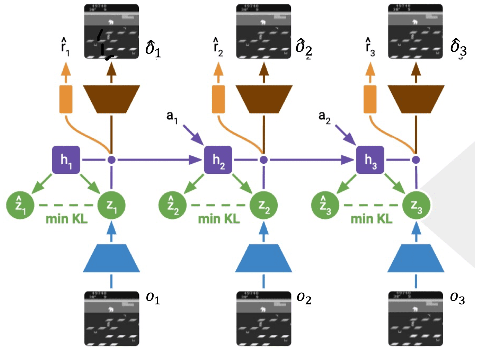
\[\mathbb{E}_{\mathrm{q}_{\phi} (\mathbf{s}_{1:T} \vert \mathbf{o}_{1:T}, \color{purple}{\mathbf{a}_{1:T}})} \left[ \sum_{t=1}^T \ln \color{red}{\mathrm{p}_{\theta} (\mathbf{o}_t \vert \mathbf{s}_t)} + \ln \color{purple}{\mathrm{p}_{\theta} (r_t \vert \mathbf{s}_t )} - \text{KL}\left[ \color{blue}{\mathrm{q}_\phi (\mathbf{s}_t \vert \mathbf{o}_{\leq t}, \color{purple}{\mathbf{a}_{< t}})} \Vert \color{green}{\mathrm{p}_{\theta} (\mathbf{s}_t \vert \mathbf{s}_{t-1}, \color{purple}{\mathbf{a}_{t-1}})} \right]\right]\]Moreover, the authors of PlaNet found that purely stochastic transitions make it difficult for the transition model to reliably remember information for multiple time steps. This motivates to introduce a deterministic sequence of activation vectors \(\{\mathbf{h}_t\}_{t=1}^T\) where \(\mathbf{h}_t\) encoding the information of \((\mathbf{o}_{< t}, \mathbf{s}_{< t}, \mathbf{a}_{< t})\), enabling the model to access not just the last state but all previous states deterministically. By extending sequential VAE to the recurrent state-space model:
- Deterministic state model: \(\mathbf{h}_t = \text{RNN}_{\theta} (\mathbf{h}_{t-1}, \mathbf{s}_{t-1}, \mathbf{a}_{t-1})\)
- Representation model (posterior): \(\mathbf{s}_t \sim \mathrm{q}_\phi (\mathbf{s}_t \vert \mathbf{h}_t, \mathbf{o}_t)\)
- Transition model (prior): \(\hat{\mathbf{s}}_t \sim \mathrm{p}_{\theta} (\mathbf{s}_t \vert \mathbf{h}_t)\)
- Observation predictor: \(\mathbf{o}_t \sim \mathrm{p}_{\theta} (\mathbf{o}_t \vert \mathbf{s}_t)\)
- Reward model: \(r_t \sim \mathrm{p}_{\theta} (r_t \vert \mathbf{s}_t)\)
where \(\mathrm{q}_{\phi} (\mathbf{s}_{1:T} \vert \mathbf{o}_{1:T}, \mathbf{a}_{1:T}) = \prod_{t=1}^T \mathrm{q}_{\phi} (\mathbf{s}_t \vert \mathbf{h}_t, \mathbf{o}_t)\).
These fundamentals underpin RSSM-based methods, serving as foundational principles. While the specifics of the training objectives may vary, these fundamental concepts are shared across different approaches.
Deep Planning Network (PlaNet)
Hafner et al. 2019 proposed PlaNet, abbreviation for deep planning network, which learns a latent environment dynamics from pixel observations and chooses actions by fast online planning in a compact latent state space. This enables the efficient behavior of the agent, reaching the performance comparable to the best model-free algorithms while using 200 times fewer episodes and similar or even less computation time.
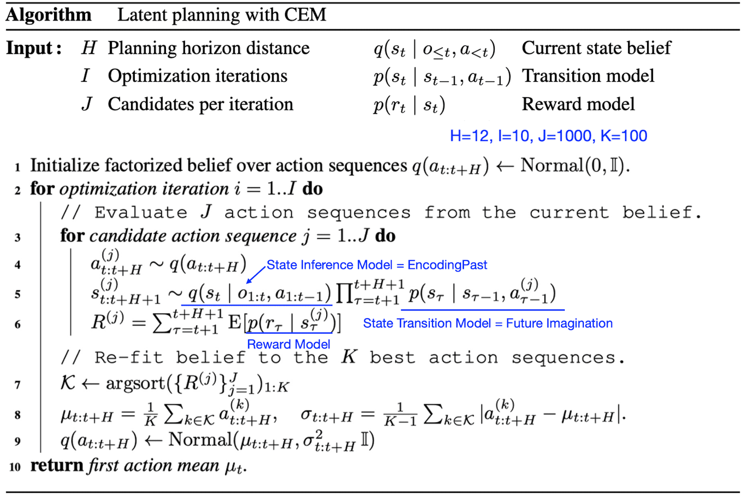
Planning with CEM
PlaNet use the cross entropy method (CEM) to search for the best action sequence under the model, and hence it falls into decision-time planning category in MBRL.
It initializes a time-dependent diagonal Gaussian over optimal action sequences
\[\mathbf{a}_{t: t+H} \sim \mathcal{N}(\mu_{t: t+H}, \sigma_{t:t+H}^2 \mathbb{I})\]where $t$ is the current timestep of the agent and $H$ is the length of the planning.
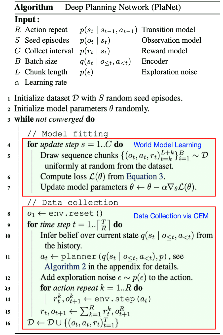
Latent Dynamics Learning
As explained in the preliminary section, PlaNet splits the hidden state into a stochastic part $\mathbf{s}_t$ and deterministic part $\mathbf{h}_t$ encoding the history \((\mathbf{o}_{< t}, \mathbf{s}_{< t}, \mathbf{a}_{< t})\) and models the following latent dynamics with the objective $\mathcal{L}(\theta)$:
\[\begin{aligned}[t] & \text{Deterministic state model} && \mathbf{h}_t = \text{RNN}_{\theta} (\mathbf{h}_{t-1}, \mathbf{s}_{t-1}, \mathbf{a}_{t-1}) \\ & \text{Stochastic state model (transition model)} && \mathbf{s}_t \sim \mathrm{p}_{\theta} (\mathbf{s}_{t} \vert \mathbf{h}_t) \\ & \text{Representation model} && \mathbf{s}_t \sim \mathrm{q}_{\phi} (\mathbf{s}_t \vert \mathbf{h}_t, \mathbf{o}_t) \\ & \text{Observation model} && \mathbf{o}_t \sim \mathrm{p}_{\theta} (\mathbf{o}_{t} \vert \mathbf{s}_{t}) \\ & \text{Reward model} && r_t \sim \mathrm{p}_{\theta} (r_t \vert \mathbf{s}_{t}) \\ \end{aligned}\] \[\mathcal{L}(\theta, \phi) = \mathbb{E}_{\mathrm{q}_{\phi} (\mathbf{s}_{1:T} \vert \mathbf{o}_{1:T}, \mathbf{a}_{1:T})} \left[ \sum_{t=1}^T \ln \mathrm{p}_{\theta} (\mathbf{o}_t \vert \mathbf{s}_t) + \ln \mathrm{p}_{\theta} (r_t \vert \mathbf{s}_t) - \text{KL}\left[ \mathrm{q}_\phi (\mathbf{s}_t \vert \mathbf{h}_{t}, \mathbf{o}_t) \Vert \mathrm{p}_{\theta} (\mathbf{s}_t \vert \mathbf{h}_{t}) \right] \right]\]where \(\mathrm{q}_{\phi} (\mathbf{s}_{1:T} \vert \mathbf{o}_{1:T}, \mathbf{a}_{1:T}) = \prod_{t=1}^T \mathrm{q}_{\phi} (\mathbf{s}_t \vert \mathbf{h}_t, \mathbf{o}_t)\).
Experimental Results
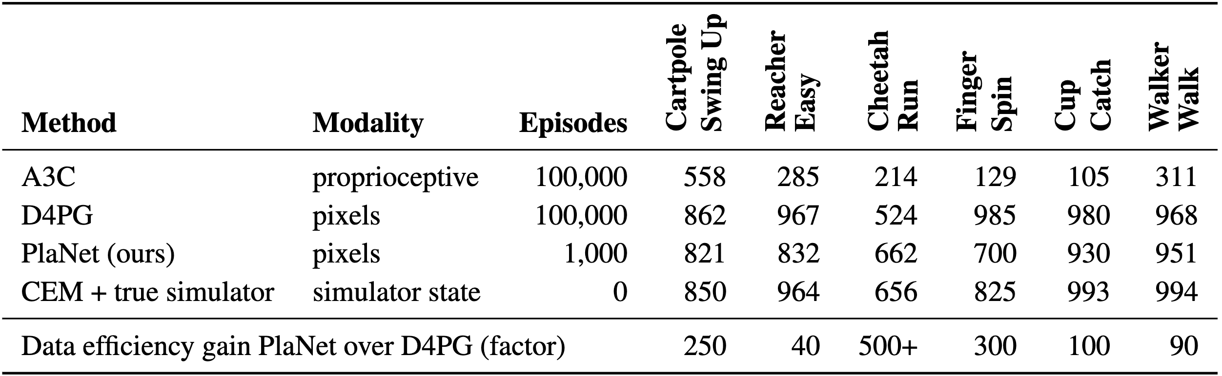
PlaNet either matches or outperforms the performance of the top model-free algorithms across 6 image-based continuous control tasks, each presenting unique challenges. Moreover, the authors noted the significance of incorporating both stochastic and deterministic elements within the transition function across all tasks in their experiments.
While the deterministic component enables the model to retain information over extended time steps, the stochastic aspect proves to be even more crucial, the agent mainly learns with the stochastic component – the agent does not learn without it. This may stem from the inherent stochasticity of the tasks from the agent’s viewpoint, occuring from the partial observability of the initial states.
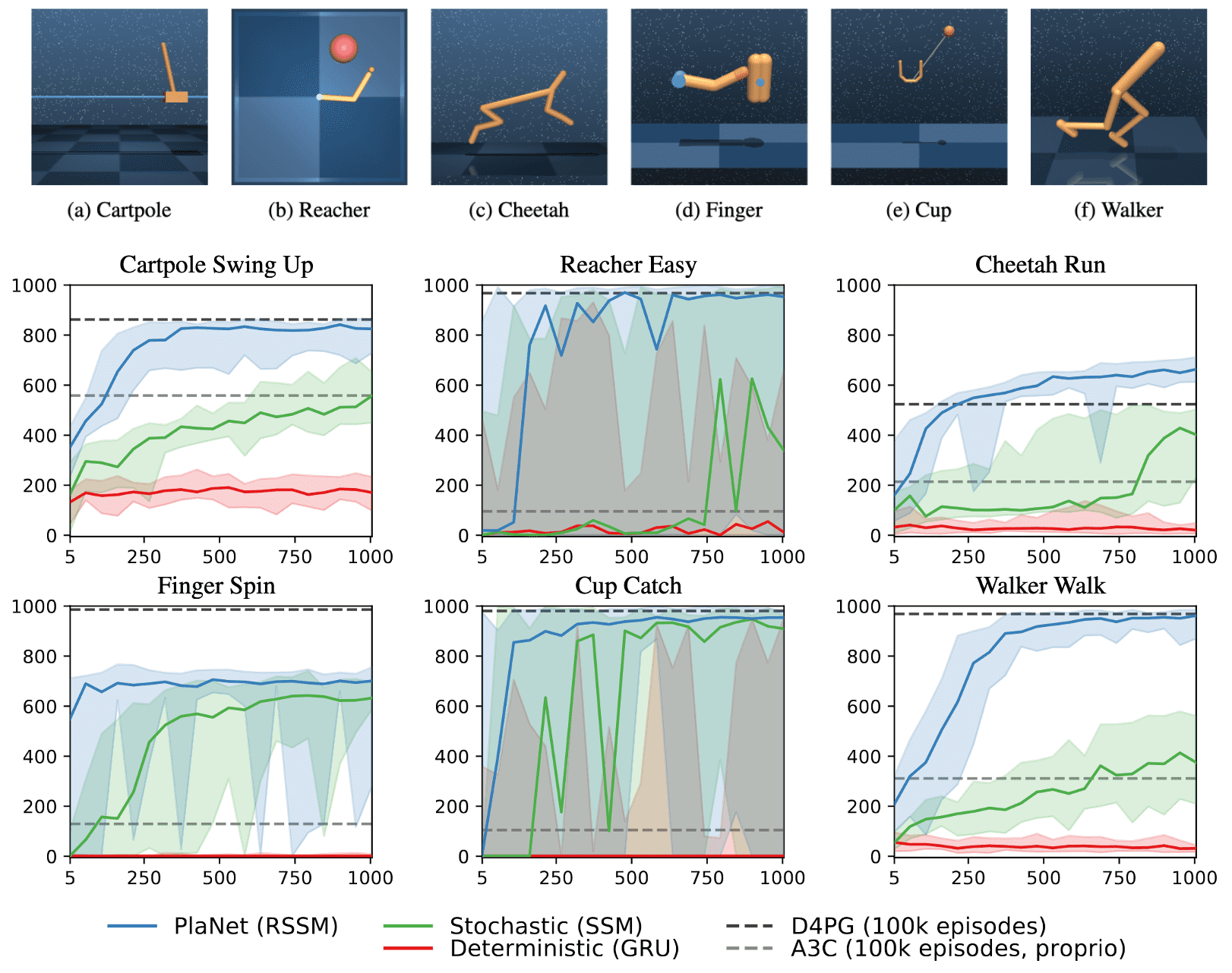
Regarding the efficiency, PlaNet outperforms the policy-gradient method A3C on all tasks, which is trained from proprioceptive states for 100,000 episodes, within only 100 episodes. Af-ter 500 episodes, it achieves performance similar to D4PG, trained from images for 100,000 episodes, except for the finger task. PlaNet surpasses the final performance of D4PG with a relative improvement of 26% on the cheetah running task.
Dreamer
Hafner et al. 2020 proposed Dreamer, an actor-critic agent learning in the imagination with the learned latent dynamics of an environment model (called world model). And the latent dynamics is learned based on collected experience, and the resulting model is shown to have the capability of performing long rollout and value estimation.
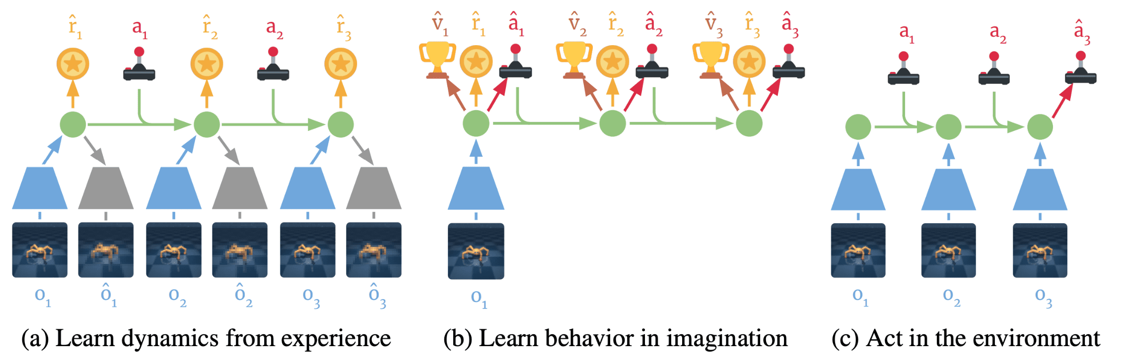
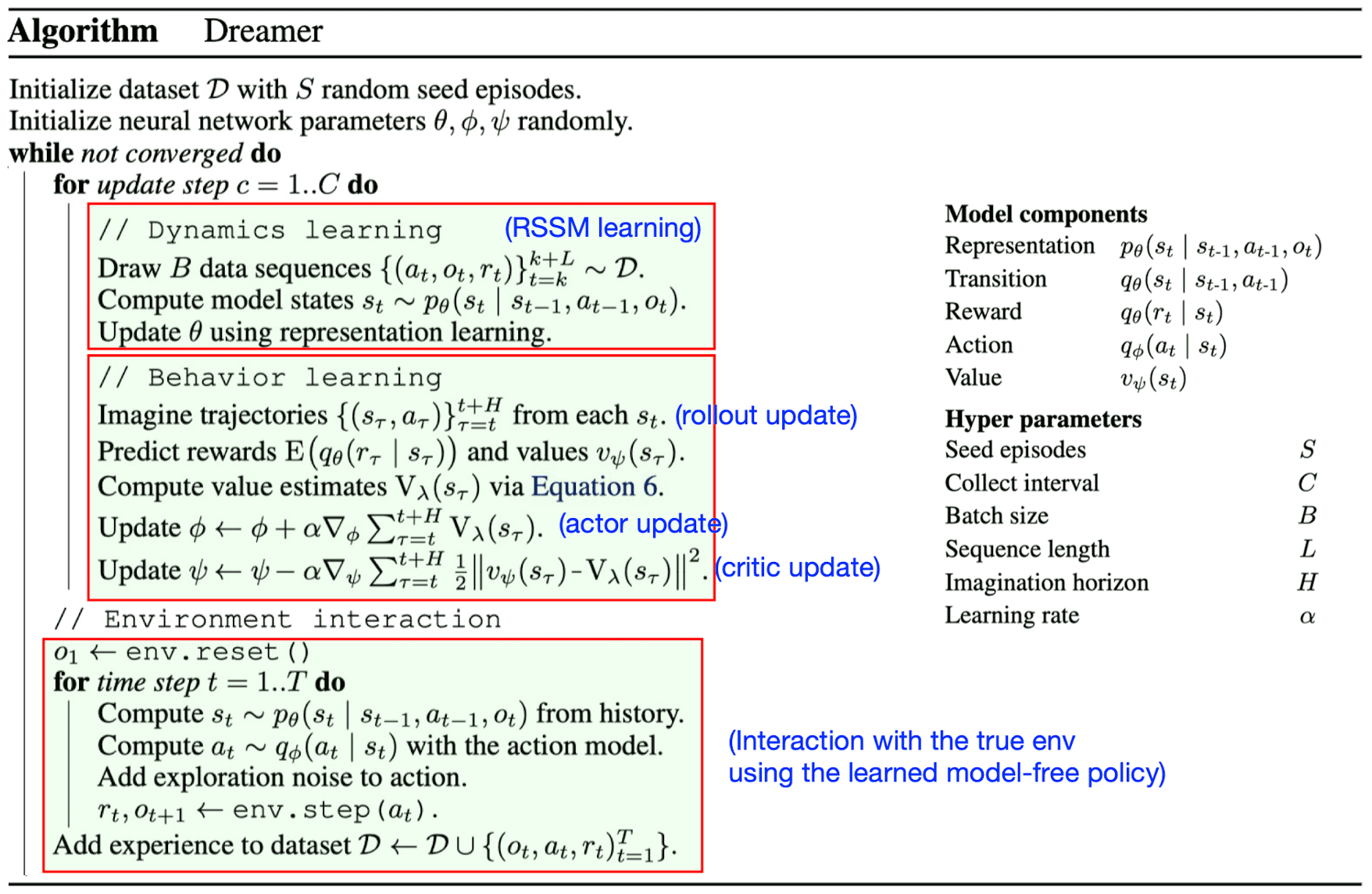
The Dreamer algorithm consists of 3 components:
- Latent Dynamics (RSSM) Learning
It learns the RSSM latent dynamics model from the dataset $\mathcal{D}$ of past experience to predict future rewards from actions and past observations. Any learning objective for the world model can be incorporated. - Behavior Learning in Imagination
It learns actor $\mathrm{q}_{\phi} (\mathbf{a}_t \vert \mathbf{s}_t)$ and critic $v_{\psi} (\mathbf{s}_t)$ from predicted latent trajectories. The value model optimizes Bellman consistency for imagined rewards and the action model is updated by propagating gradients of value estimates back through the neural network dynamics. - True Environment Interaction
It collects new experience for $\mathcal{D}$ by executing the learned actor in the true world.
Latent Dynamics Learning
To learn the latent, any learning objective can be incorporated. One of the fine selection explored by authors is RSSM learning with the following world model components, dictating the notation of the original paper:
\[\begin{aligned}[t] & \text{Deterministic state model} && \mathbf{h}_t = \text{RNN}_\theta (\mathbf{h}_{t−1}, \mathbf{s}_{t−1}, \mathbf{a}_{t−1}) \\ & \text{Representation model} && \mathbf{s}_t \sim \mathrm{p}_\theta (\mathbf{s}_t \vert \mathbf{h}_t, \mathbf{o}_t) \\ & \text{Observation model} && \mathbf{o}_t \sim \mathrm{q}_\theta (\mathbf{o}_t \vert \mathbf{s}_t) \\ & \text{Reward model} && r_t \sim \mathrm{q}_\theta (r_t \vert \mathbf{s}_t) \\ & \text{Transition model} && \mathbf{s}_t \sim \mathrm{q}_\theta (\mathbf{s}_t \vert \mathbf{h}_{t}) \\ \end{aligned}\] \[\mathcal{L}(\theta) = \mathbb{E}_{\mathrm{p}_{\theta} (\mathbf{s}_{1:T} \vert \mathbf{o}_{1:T}, \mathbf{a}_{1:T})} \left[ \sum_{t=1}^T \ln \mathrm{q}_{\theta} (\mathbf{o}_t \vert \mathbf{s}_t) + \ln \mathrm{q}_{\theta} (r_t \vert \mathbf{s}_t) - \beta \cdot \text{KL}\left[ \mathrm{p}_\theta (\mathbf{s}_t \vert \mathbf{h}_t, \mathbf{o}_t) \Vert \mathrm{q}_\theta (\mathbf{s}_t \vert \mathbf{h}_{t}) \right] \right]\]where \(\mathrm{p}_{\theta} (\mathbf{s}_{1:T} \vert \mathbf{o}_{1:T}, \mathbf{a}_{1:T}) = \prod_{t=1}^T \mathrm{p}_{\theta} (\mathbf{s}_t \vert \mathbf{h}_t, \mathbf{o}_t)\). However, predicting pixels from the hidden latent state can require high model capacity. Instead, it is possible to circumvent the generation of pixels by predicting the states from the images, replacing the observation model \(\mathrm{q}_\theta (\mathbf{o}_t \vert \mathbf{s}_t)\) with the state model \(\mathrm{q}_\theta (\mathbf{s}_t \vert \mathbf{o}_t)\). By subtracting the constant marginal probability \(\ln \mathrm{q}(\mathbf{o}_t)\) of the data under the variational encoder \(\mathrm{p}_{\theta} (\mathbf{s}_{1:T} \vert \mathbf{o}_{1:T}, \mathbf{a}_{1:T})\), Bayes’ rule and the InfoNCE mini-batch bound provide the following inequality:
\[\begin{aligned} \mathbb{E}_{\mathrm{p}_{\theta} (\mathbf{s}_{1:T} \vert \mathbf{o}_{1:T}, \mathbf{a}_{1:T})} \left[ \ln \mathrm{q}_{\theta} (\mathbf{o}_t \vert \mathbf{s}_t) \right] & = \mathbb{E}_{\mathrm{p}_{\theta} (\mathbf{s}_{1:T} \vert \mathbf{o}_{1:T}, \mathbf{a}_{1:T})} \left[ \ln \mathrm{q}_{\theta} (\mathbf{o}_t \vert \mathbf{s}_t) - \ln q_{\theta} (\mathbf{o}_t) \right] \\ & = \mathbb{E}_{\mathrm{p}_{\theta} (\mathbf{s}_{1:T} \vert \mathbf{o}_{1:T}, \mathbf{a}_{1:T})} \left[ \ln \mathrm{q}_{\theta} (\mathbf{s}_t \vert \mathbf{o}_t) - \ln q_{\theta} (\mathbf{s}_t) \right] \\ & \geq \mathbb{E}_{\mathrm{p}_{\theta} (\mathbf{s}_{1:T} \vert \mathbf{o}_{1:T}, \mathbf{a}_{1:T})} \left[ \ln \mathrm{q}_{\theta} (\mathbf{s}_t \vert \mathbf{o}_t) - \ln \sum_{\mathbf{o}^\prime} q_{\theta} (\mathbf{s}_t \vert \mathbf{o}^\prime) \right] \\ \end{aligned}\]Intuitively, \(\mathrm{q}_{\theta} (\mathbf{s}_t \vert \mathbf{o}_t)\) makes the state predictable from the current image while \(\ln \sum_{\mathbf{o}^\prime} q_{\theta} (\mathbf{s}_t \vert \mathbf{o}^\prime)\) keeps it diverse to prevent collapse. Hence, the contrastive version of Dreamer objective is given by
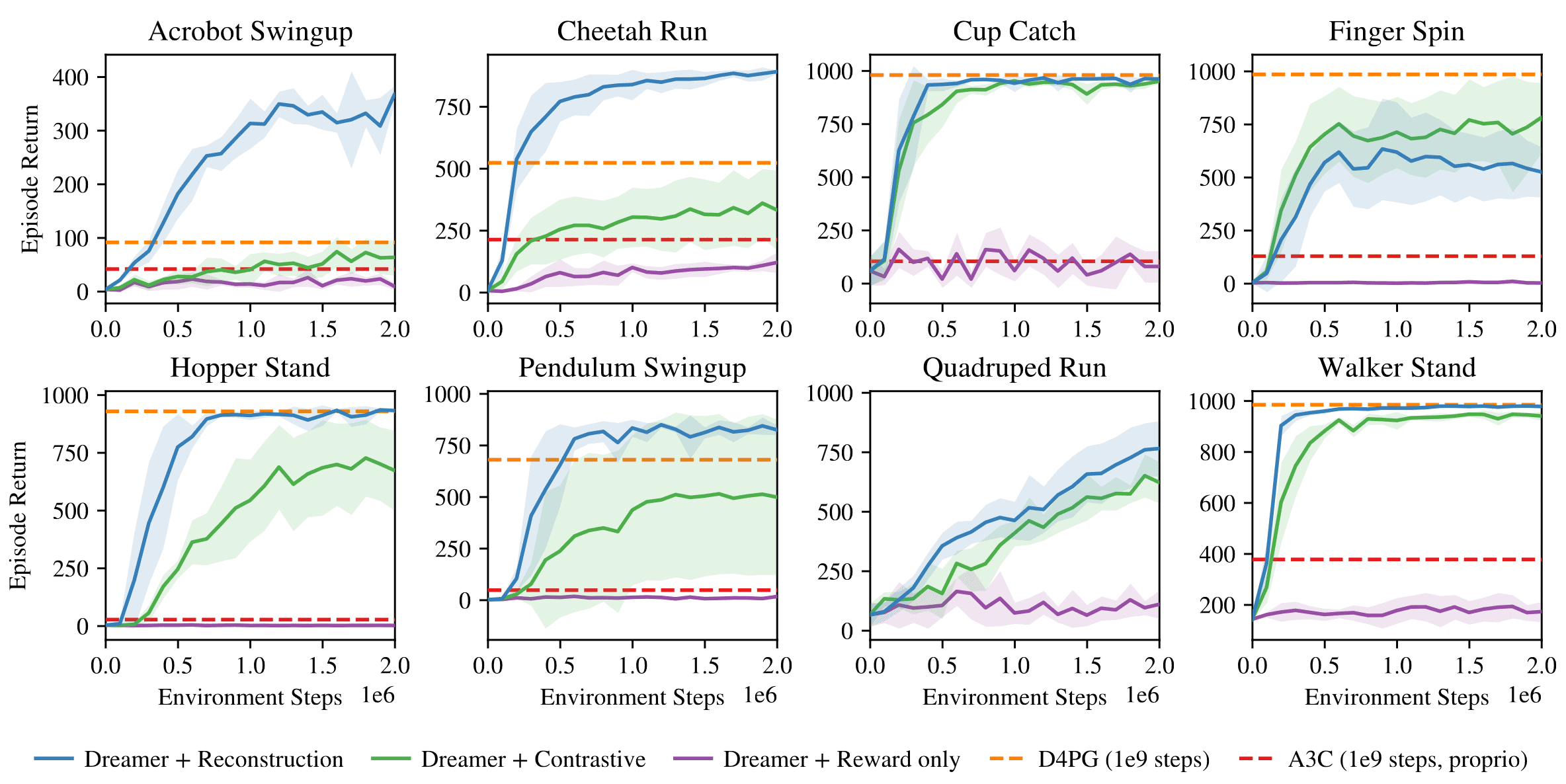
\[\mathcal{L}(\theta) = \mathbb{E}_{\mathrm{p}_{\theta} (\mathbf{s}_{1:T} \vert \mathbf{o}_{1:T}, \mathbf{a}_{1:T})} \left[ \sum_{t=1}^T \ln \mathrm{q}_{\theta} (\mathbf{s}_t \vert \mathbf{o}_t) - \ln \sum_{\mathbf{o}^\prime} q_{\theta} (\mathbf{s}_t \vert \mathbf{o}^\prime) + \ln \mathrm{q}_{\theta} (r_t \vert \mathbf{s}_t) - \beta \cdot \text{KL}\left[ \mathrm{p}_\theta (\mathbf{s}_t \vert \mathbf{h}_t, \mathbf{o}_t) \Vert \mathrm{q}_\theta (\mathbf{s}_t \vert \mathbf{h}_{t}) \right] \right]\]However, the authors empirically observed that RSSM pixel reconstruction objective is viable, outperforming contrastive objective on most control tasks.
Actor-Critic Learning in Imagination
In the latent space of the learned world model, Dreamer uses an actor-critic approach to learn long-horizon behaviors that consider rewards beyond the horizon:
- Actor \(\mathbf{a}_t \sim \mathrm{q}_\phi (\mathbf{a}_t \vert \mathbf{s}_t) = \tanh (\mu_{\phi} (\mathbf{s}_t) + \sigma_{\phi} (\mathbf{s}_t) \varepsilon)\) where $\varepsilon \sim \mathcal{N}(\mathbf{0}, \mathbb{I})$
- Critic \(v_{\psi} (\mathbf{s}_t) \approx \mathbb{E}_{\mathbf{a}_t \sim q_\phi (\mathbf{a}_t \vert \mathbf{s}_t)} \left[ \sum_{t=1}^T \gamma^t r_t \right]\)
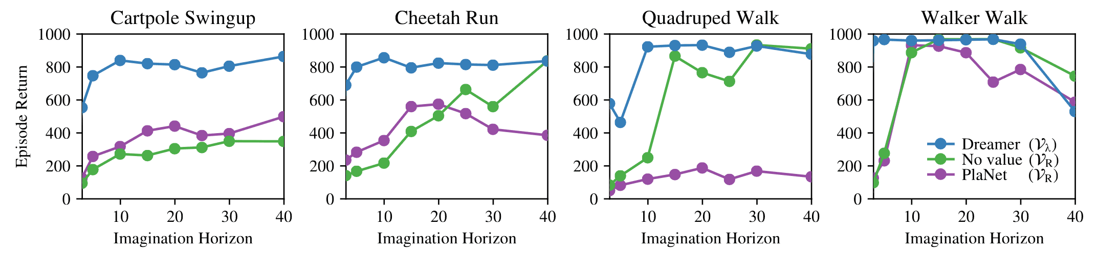
To update the action and value models, we first compute the value estimates \(V_\lambda (\mathbf{s}_{t^\prime})\), an exponentially-weighted average of the estimates for different $n$-step return to balance bias and variance for all states \(\mathbf{s}_{t^\prime}\) along the imagined trajectories \(\{ \mathbf{s}_{t^\prime}, \mathbf{a}_{t^\prime}, r_{t^\prime}\}_{t^\prime = t}^{t + H}\):
\[\mathrm{V}_{\lambda} (\mathbf{s}_t) = (1 - \lambda) \sum_{n=1}^{H-1} \lambda^{n-1} \mathrm{V}_{\mathrm{N}}^n (\mathbf{s}_t) + \lambda^{H-1} \mathrm{V}_{\mathrm{N}}^H (\mathbf{s}_t)\]where
\[\mathrm{V}_{\mathrm{N}}^n (\mathbf{s}_t) = \mathbb{E}_{\mathrm{q}_\theta, \mathrm{q}_{\phi}} \left[ \sum_{t^{\prime} = t}^{h-1} \gamma^{k - t} r_{t^\prime} + \gamma^{h - t} v_{\psi} (\mathbf{s}_h) \right] \text{ with } h = \min(t + n, t + H)\]This value estimates enables the Dreamer to be more robust to the horizon length and performs well even for short horizons, outperforming PlaNet using online planning.
Then, the objective for the actor \(\mathrm{q}_{\phi}\) is to predict actions that result in state trajectories with high value estimates, and the objective for the value model $v_\psi$, in turn, is to regress the value estimates:
\[\begin{aligned} & \text{Actor:} \quad \phi^* = \underset{\phi}{\text{argmax}} \; \mathbb{E}_{\mathrm{q}_\theta, \mathrm{q}_\phi} \left[ \sum_{t^\prime = t}^{t + H} \mathrm{V}_{\lambda} (\mathbf{s}_{t^\prime}) \right] \\ & \text{Critic:} \quad \psi^* = \underset{\psi}{\text{argmin}} \; \mathbb{E}_{\mathrm{q}_\theta, \mathrm{q}_\phi} \left[ \sum_{t^\prime = t}^{t + H} \frac{1}{2} \lVert v_{\psi}(\mathbf{s}_{t^\prime}) - \mathrm{V}_{\lambda} (\mathbf{s}_{t^\prime}) \rVert^2 \right] \end{aligned}\]The world model is fixed while learning behaviors. The overall pseudocode of Dreamer is illustrated in the following figure.
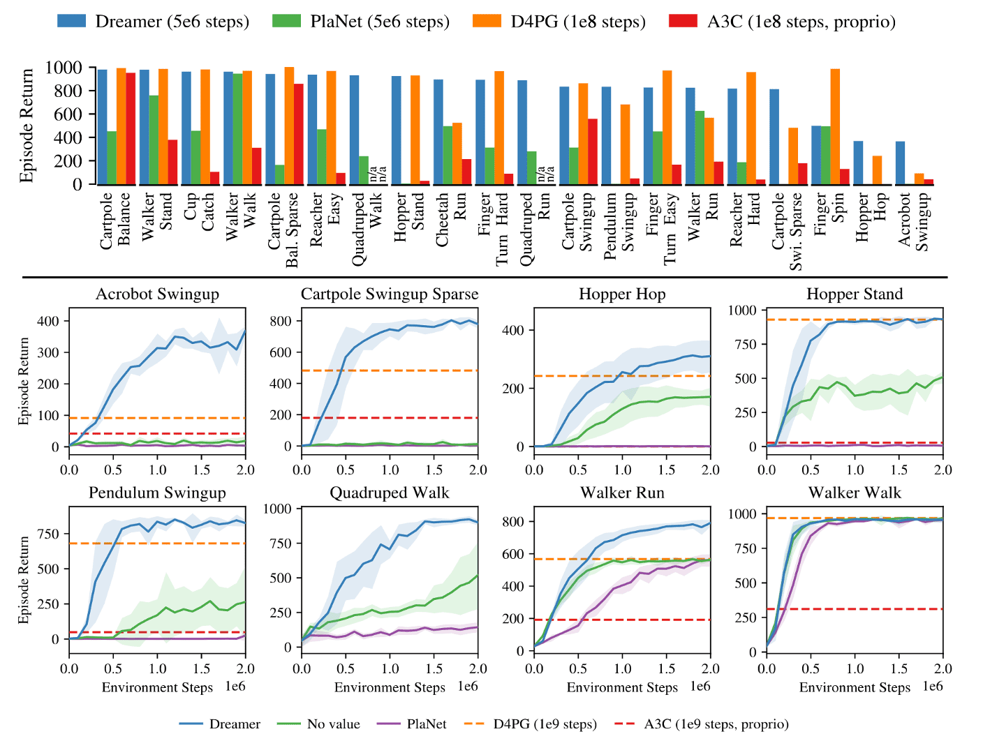
Experimental Results
The authors compared Dreamer to state-of-the-art RL agents on 20 visual control tasks. After $5 \times 10^6$ environment steps, Dreamer reaches an average performance of $823$ across tasks, exceeding the performance of PlaNet at $332$ and the top model-free D4PG agent at $786$ after $108$ steps. Furthermore, Dreamer turns out to be more robust to the horizon and performs well even for short horizons.
Simultaneously, Dreamer inherits the data efficiency of PlaNet, confirming that the learned world model aids in generalizing from small amounts of experience. The empirical success of Dreamer highlights that learning behaviors via latent imagination with world models can surpass top methods based on experience replay.
DreamerV2
Hafner et al. 2021 further proposed DreamerV2 that supports the agent to learn purely from rollout data of the separately trained world model and firstly achieve human-level performance on 55 Atari game tasks. Compared with Dreamer, DreamerV2 replaces the Gaussian latent as proposed in PlaNet with the discrete latent, which brings superior performance. The possible reason for such effects would be the discrete latent representation can better fit the aggregate posterior and handle multi-modal cases.
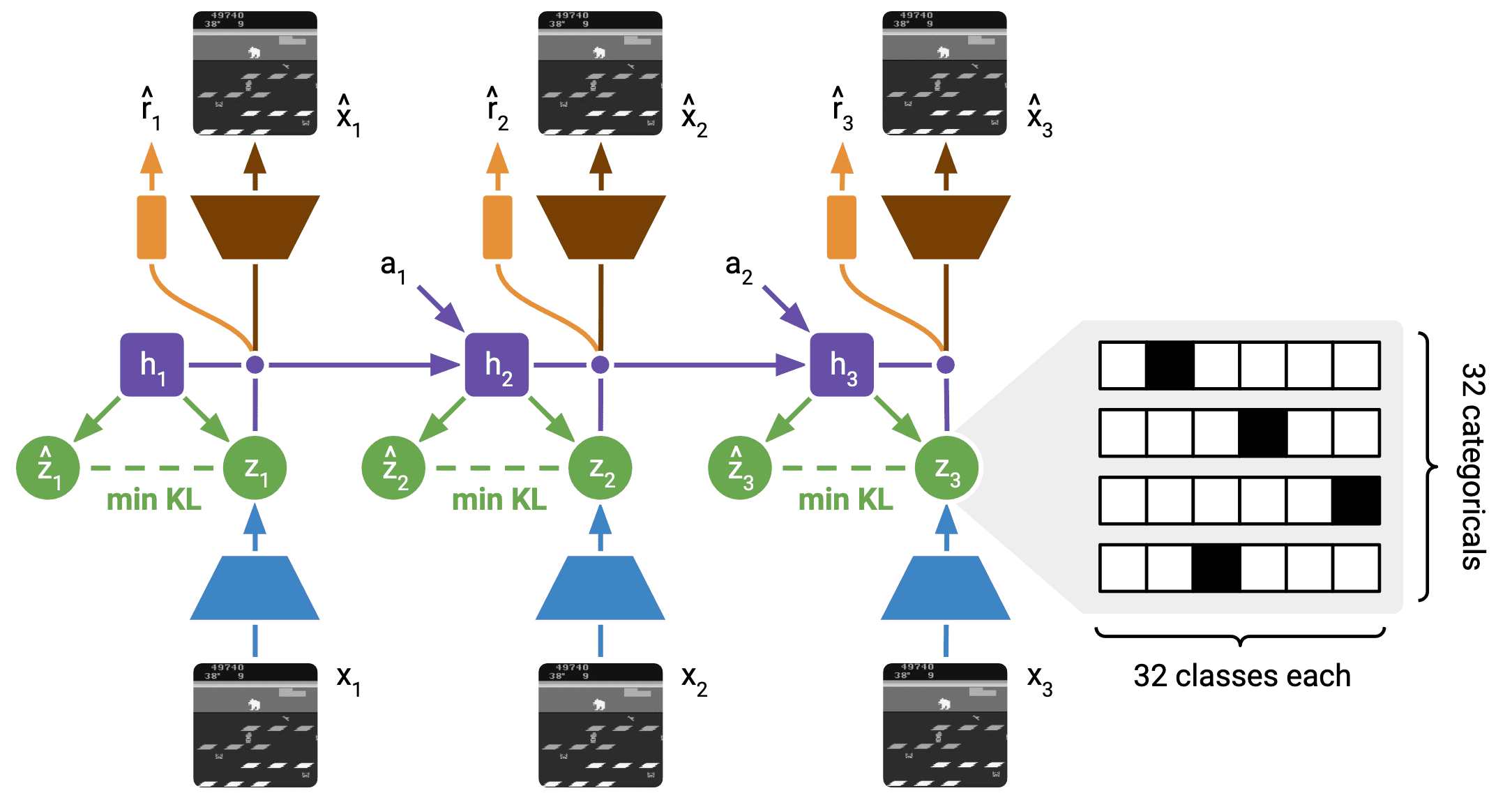
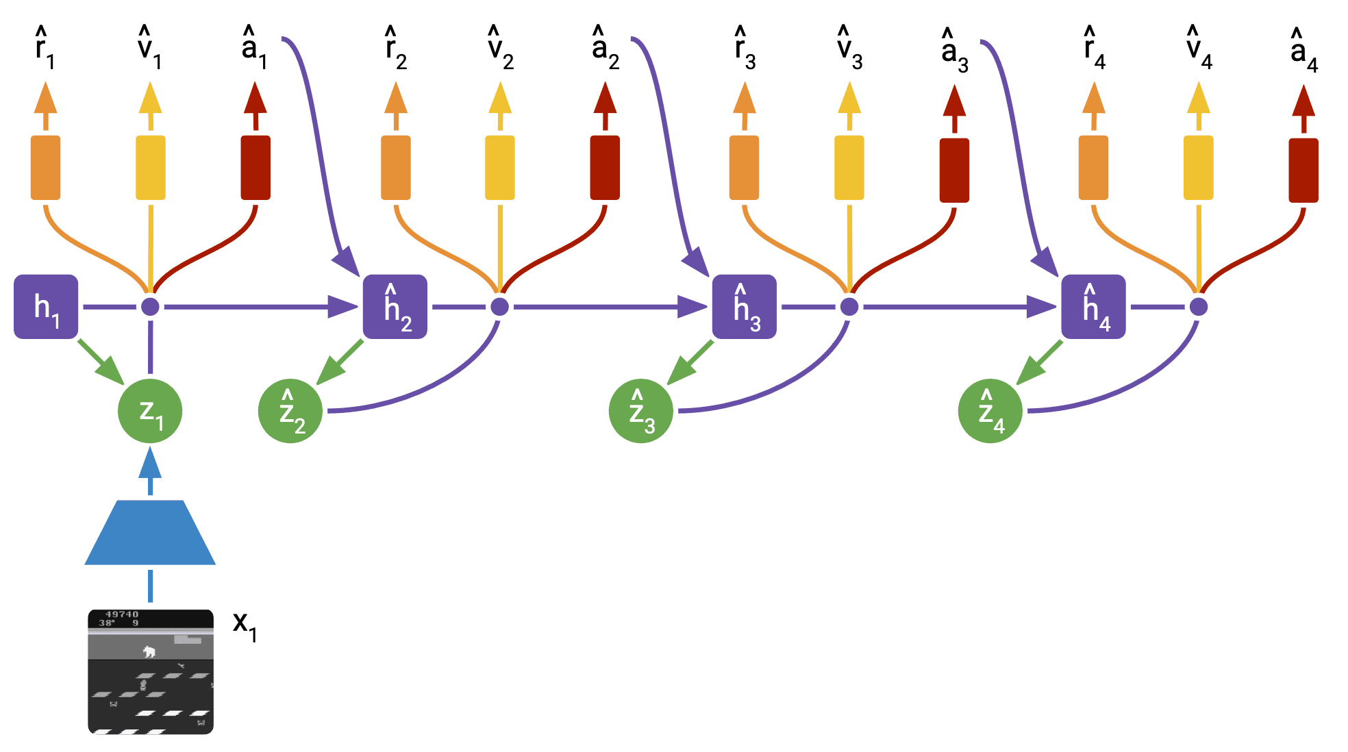
Latent Dynamics Learning
The world model of DreamerV2 consists of an image encoder, a RSSM to learn the dynamics, and predictors for the image, reward, and discount factor. Note that the posterior state \(\mathbf{s}_t\) incorporates information about the current image \(\mathbf{o}_t\), while the prior state \(\hat{\mathbf{s}}_t\) aims to predict the posterior without access to the current image. Unlike in PlaNet and DreamerV1, the stochastic state of DreamerV2 is a vector of multiple categorical variables.
\[\begin{aligned}[t] & \text{Recurrent model:} && \mathbf{h}_t = \text{RNN}_\theta (\mathbf{h}_{t-1}, \mathbf{s}_{t-1}, \mathbf{a}_{t-1}) \\ & \text{Representation model:} && \mathbf{s}_t \sim \mathrm{q}_\theta (\mathbf{s}_t \vert \mathbf{h}_t, \mathbf{o}_t) \\ & \text{Transition predictor:} && \hat{\mathbf{s}}_t \sim \mathrm{p}_\theta (\hat{\mathbf{s}}_t \vert \mathbf{h}_t) \\ & \text{Image predictor:} && \hat{\mathbf{o}}_t \sim \mathrm{p}_\theta (\hat{\mathbf{o}}_t \vert \mathbf{h}_t, \mathbf{s}_t) \\ & \text{Reward predictor:} && \hat{r}_t \sim \mathrm{p}_\theta (\hat{r}_t \vert \mathbf{h}_t, \mathbf{s}_t) \\ & \text{Discount predictor:} && \hat{\gamma}_t \sim \mathrm{p}_\theta (\hat{\gamma}_t \vert \mathbf{h}_t, \mathbf{s}_t). \end{aligned}\] \[\mathcal{L}(\theta) = \mathbb{E}_{\mathrm{q}_{\theta} (\mathbf{s}_{1:T} \vert \mathbf{o}_{1:T}, \mathbf{a}_{1:T})} \left[ \sum_{t=1}^T \ln \mathrm{p}_\theta (\hat{\mathbf{o}}_t \vert \mathbf{h}_t, \mathbf{s}_t) + \ln \mathrm{p}_\theta (\hat{r}_t \vert \mathbf{h}_t, \mathbf{s}_t) + \ln \mathrm{p}_\theta (\hat{\gamma}_t \vert \mathbf{h}_t, \mathbf{s}_t) - \beta \cdot \text{KL}\left[ \mathrm{q}_\theta (\mathbf{s}_t \vert \mathbf{h}_t, \mathbf{o}_t) \Vert \mathrm{p}_\theta (\hat{\mathbf{s}}_t \vert \mathbf{h}_{t}) \right] \right]\]where $\theta$ denotes their combined parameter vector and \(\mathrm{q}_{\theta} (\mathbf{s}_{1:T} \vert \mathbf{o}_{1:T}, \mathbf{a}_{1:T}) = \prod_{t=1}^T \mathrm{q}_{\theta} (\mathbf{s}_t \vert \mathbf{h}_t, \mathbf{o}_t)\).
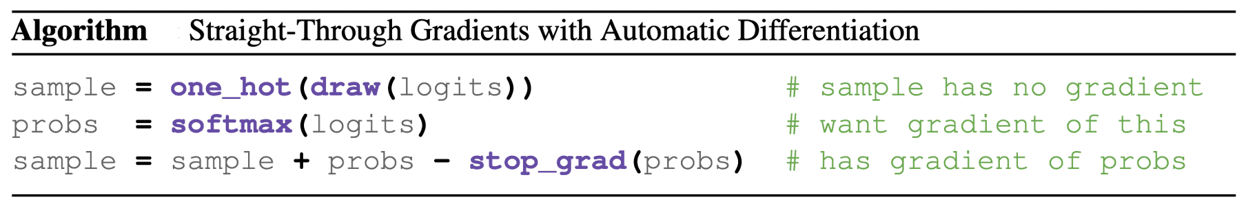
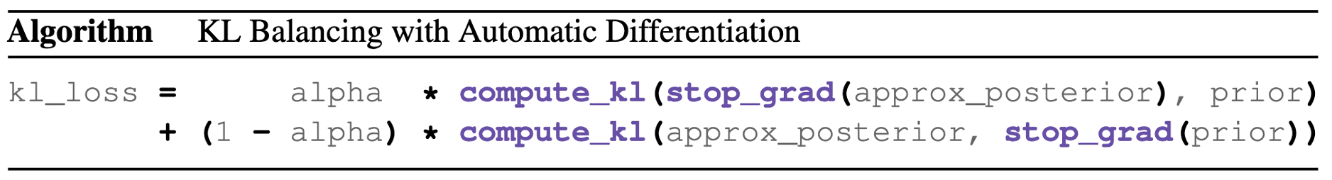
To optimize the discrete categorical latent states, straight-through gradients can be easily easy implemented via automatic differentiation.
Moreover, to avoid regularizing the representations toward a poorly trained prior, the authors utilized KL balancing that minimizes the KL loss faster with respect to the prior than the representations by using different learning rates, $\alpha = 0.8$ for the prior and $1 − \alpha$ for the approximate posterior.
Actor-Critic Learning
To learn long-horizon behaviors in the imagination MDP, DreamerV2 harnesses stochastic actor and deterministic critic. The actor aims to generate actions that lead to states that optimize the critic output, and the critic aims to accurately estimate the cumulative rewards expected from the actions of the actor from each imagined state.
\[\begin{aligned}[t] & \text{Actor:} && \hat{\mathbf{a}}_t \sim \mathrm{p}_\phi (\hat{\mathbf{a}}_t \vert \hat{\mathbf{s}}_t) \\ & \text{Critic:} && v_\psi (\hat{\mathbf{s}}_t) \approx \mathbb{E}_{\mathrm{p}_\theta, \mathrm{p}_\phi} \left[ \sum_{t^\prime \geq t} \hat{\gamma}^{t^\prime - t} \hat{r}_t \right] \end{aligned}\]Note that the actor also outputs a categorical distribution over actions.
Critic loss function
Instead of 1-step target that sums the current reward and the critic output for the following state, DreamerV2 inherits $\lambda$-target used in Dreamer, which is recursively defined by:
\[V_t^\lambda \doteq \hat{r}_t + \hat{\gamma}_t \begin{cases} (1-\lambda) v_{\xi}\left(\hat{\mathbf{s}}_{t+1}\right)+\lambda V_{t+1}^\lambda & \text { if } t<H \\ v_{\psi}\left(\hat{\mathbf{s}}_H\right) & \text { if } t=H \end{cases}\]In practice, $\lambda = 0.95$ to focus more on long horizon targets than on short horizon targets. Then, the critic is trained to regress the $\lambda$-return using a squared loss:
\[\mathcal{L}(\psi) \doteq \mathbb{E}_{\mathrm{p}_\theta, \mathrm{p}_{\phi}} \left[ \sum_{t=1}^{H-1} \frac{1}{2} \left( v_\psi ( \hat{\mathbf{s}}_t) - \text{sg} \left( V_t^\lambda \right) \right)^2 \right]\]Moreover, the authors further stabilized value learning with a target network in DQN. Specifically, the targets are computed using a copy of the critic that is updated every 100 gradient steps.
Actor loss function
The actor aims to output actions that maximize the prediction of long-term future rewards made by the critic. DreamerV2 combines unbiased but high-variance REINFORCE gradients with biased but low-variance straight-through gradients. Moreover, it regularizes the entropy of the actor to encourage exploration where feasible while allowing the actor to choose precise actions when necessary.
\[\mathcal{L}(\phi) \doteq \mathrm{E}_{\mathrm{p}_\theta, \mathrm{p}_\phi} \left[\sum_{t=1}^{H-1}\left\{\underbrace{-\rho \ln \mathrm{p}_\phi\left(\hat{\mathbf{a}}_t \mid \hat{\mathbf{s}}_t\right) \operatorname{sg}\left(V_t^\lambda-v_{\psi}\left(\hat{\mathbf{s}}_t\right)\right)}_{\text {REINFORCE }} \underbrace{-(1-\rho) V_t^\lambda}_{\substack{\text { dynamics } \\ \text { backprop }}} \underbrace{-\eta \cdot \mathrm{H}\left[\mathrm{a}_t \mid \hat{\mathbf{s}}_t\right]}_{\text {entropy regularizer }}\right\} \right]\]Intuitively, the low-variance but biased dynamics backpropagation could learn faster initially and the unbiased but high-variance could to converge to a better solution. For Atari, the authors found that REINFORCE gradients to work substantially better and use $\rho = 1$. In contrast, for continuous control, $\rho = 0$ (dynamics backpropagation) works substantially.
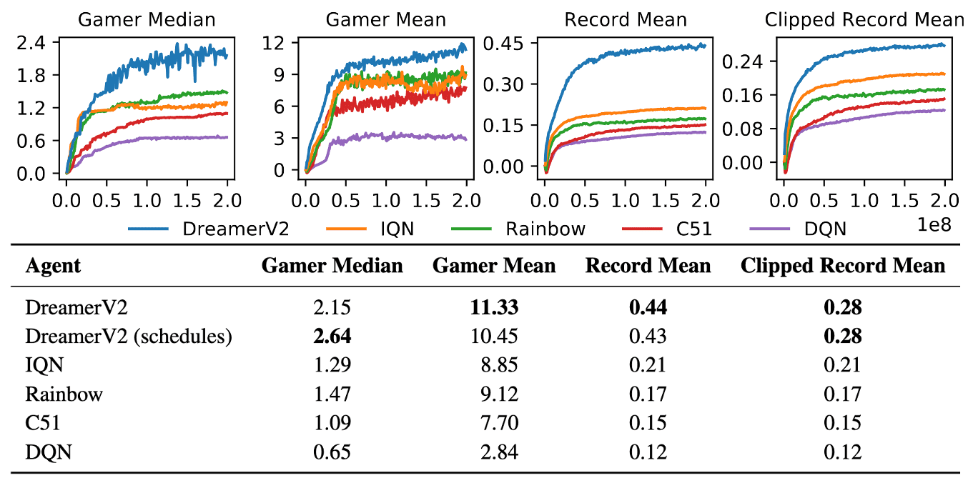
Experimental Results
As a result, DreamerV2 outperforms 4 strong model-free algorithms in all Atari benchmark with sticky actions.
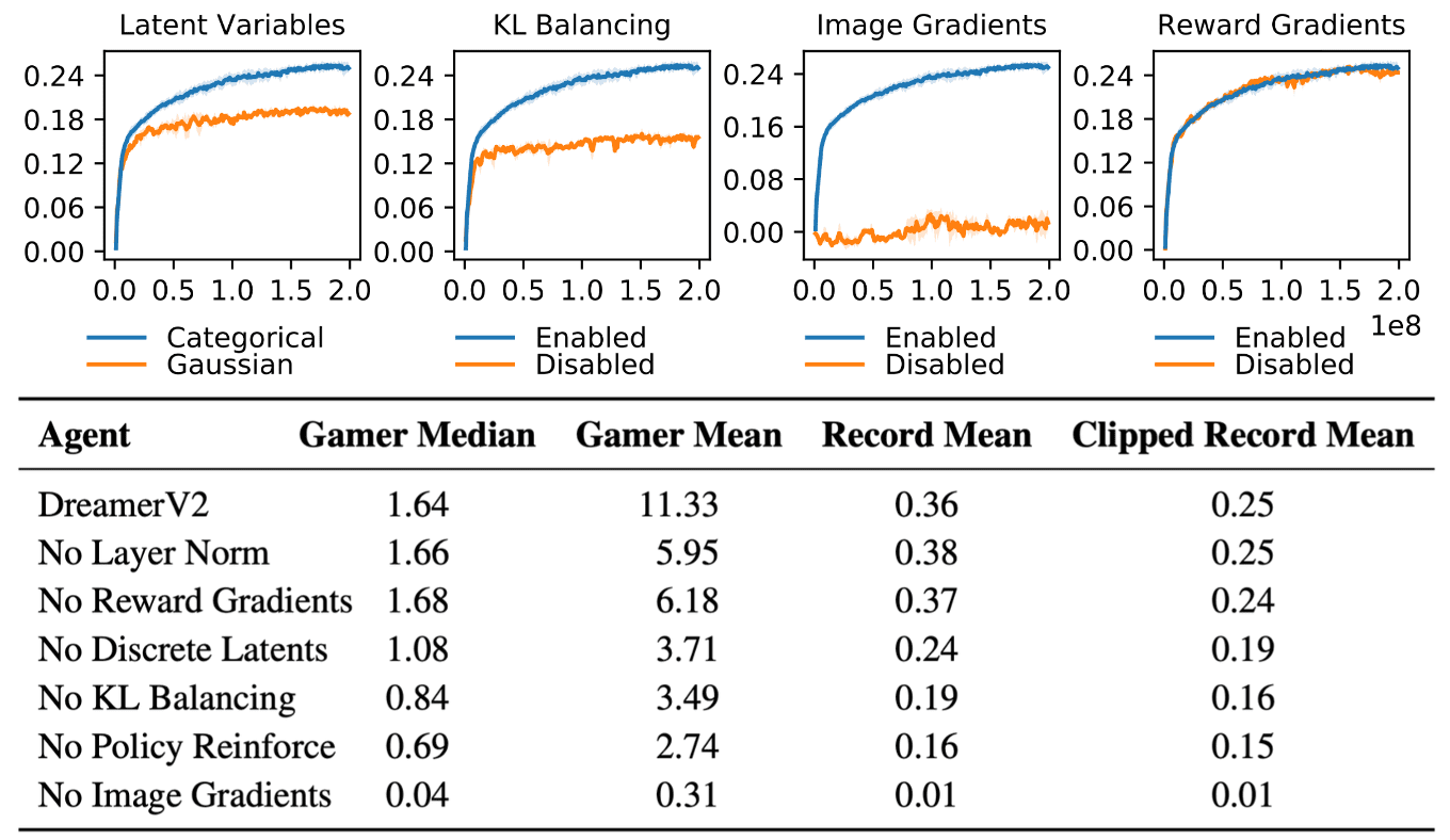
Additionally, in the ablation study, categorical latent variables outperform Gaussian latent variables in 42 out of 55 tasks. This superiority may be attributed to the following hypotheses:
- A categorical prior can seamlessly accommodate the aggregate posterior, as a mixture of categoricals forms another categorical. Conversely, a Gaussian prior struggles to align with a mixture of Gaussian posteriors, complicating the prediction of multi-modal changes between successive images.
- The sparsity level enforced by a vector of categorical latent variables could be beneficial for generalization. The compression of the 32 categorical samples, each with 32 classes, yields a sparse binary vector of length 1024 with 32 active bits.
- Contrary to common intuition, categorical variables may be easier to optimize than Gaussian variables, possibly because the straight-through gradient estimator ignores a term that would otherwise scale the gradient. This potentially mitigates issues with exploding and vanishing gradients.
- Categorical variables could provide a better inductive bias compared to unimodal continuous latent variables for capturing the non-smooth aspects of Atari games, such as when entering a new room, or when collected items or defeated enemies disappear from the image.
DreamerV3
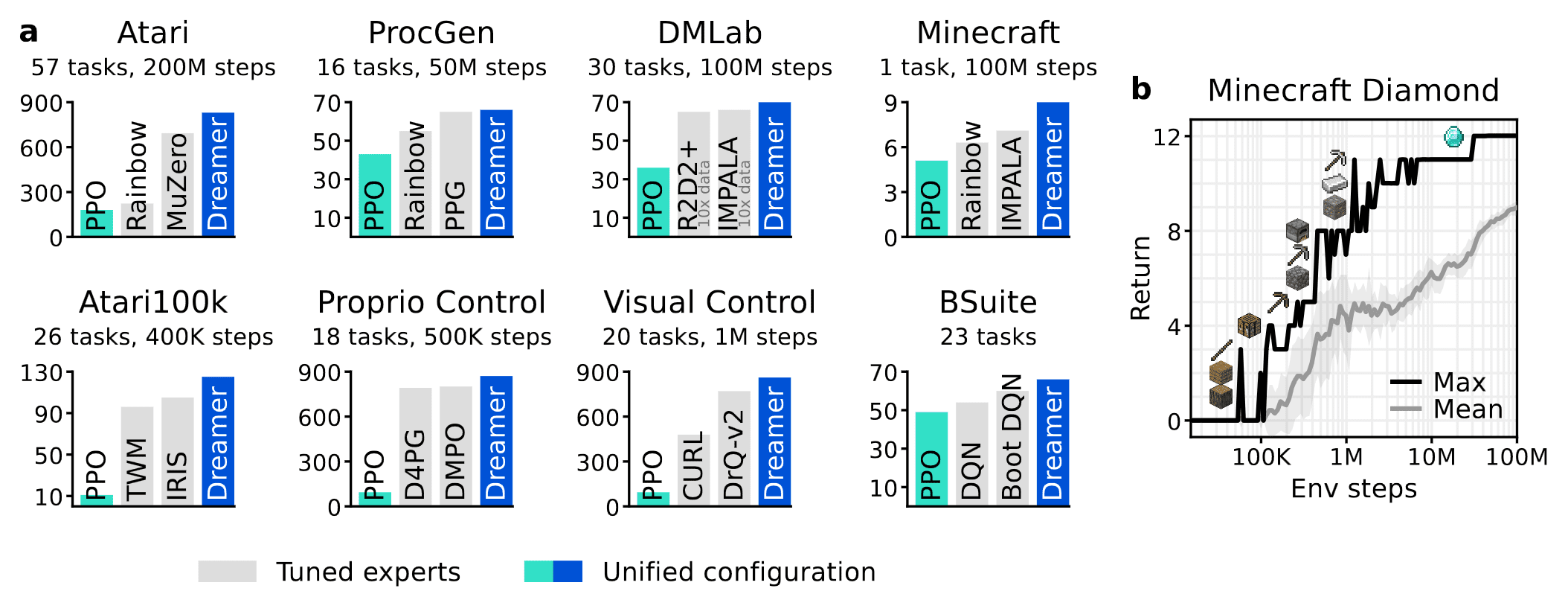
Finally, DreamerV3 is a general algorithm that learns to master diverse domains while using fixed hyperparameters, outperforming other pecialized methods with the favorable scaling properties. Consequently, DreamerV3 is the first algorithm to collect diamonds in Minecraft from scratch without human data or curricula. This achievement has been posed as a significant challenge in AI that requires exploring farsighted strategies from pixels and sparse rewards in an open world.
Key Differences
Comparing to DreamerV2, DreamerV3 is equipped with a range of robustness techniques based on normalization, balancing, and transformations:
-
Symlog predictions
Inputs to the world model are symlog-encoded and use symlog predictions with squared error for reconstructing inputs. $$ \mathrm{symlog}(x) = \mathrm{sign}(x) \ln (\vert x \vert + 1) \text{ and } \mathrm{symexp}(x) = \mathrm{sign}(x) \left( \exp (\vert x \vert) - 1 \right) $$ -
World model regularizer
Combined KL balancing with free bits technique. -
Policy regularizer
Using a fixed entropy regularizer for the actor was challenging when targeting both dense and sparse rewards. Scaling large return ranges down to the $[0, 1]$ interval, without amplifying near-zero returns, overcame this challenge. -
Unimix categoricals
We parameterize the categorical distributions for the world model representations and dynamics, as well as for the actor network, as mixtures of 1% uniform and 99% neural network output 68,69 to ensure a minimal amount of probability mass on every class and thus keep log probabilities and KL divergences well behaved. -
Critic EMA regularizer
We compute $\lambda$-returns using the fast critic network and regularize the critic outputs towards those of its own weight EMA instead of computing returns using the slow critic. -
Replay buffer
DreamerV2 used a replay buffer that only replays time steps from completed episodes. To shorten the feedback loop, DreamerV3 uniformly samples from all inserted subsequences of size batch length regardless of episode boundaries.
The following figure shows the training process of DreamerV3. The overall framework is identical to Dreamer & DreamerV2.
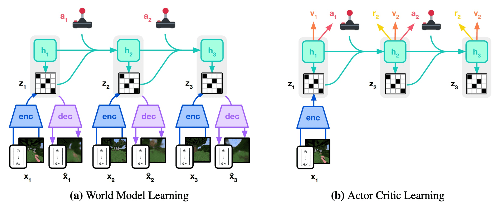
World Model Learning
For world model learning, DreamerV3 replaces the discount predictor by continue predictor \(c_t \sim \mathrm{p}_{\theta} (c_t \vert \mathbf{h}_t, \mathbf{s}_t)\) where \(c_t \in \{ 0, 1 \}\) is an episode continutation flags. The world model parameters $\theta$s are optimized end-to-end to maximize the following objective (in practice, $\beta_{\text{pred}} = 1$, $\beta_{\text{dyn}} = 1$, and $\beta_{\text{rep}} = 0.1$):
\[\begin{gathered} \mathcal{L}(\theta) = \mathbb{E}_{q_\theta} \left[ \sum_{t=1}^T ( \beta_{\text{pred}} \mathcal{L}_{\text{pred}} (\theta) + \beta_{\text{dyn}} \mathcal{L}_{\text{dyn}} (\theta) + \beta_{\text{rep}} \mathcal{L}_{\text{rep}} (\theta) )\right] \\ \begin{aligned} \text{ where } \mathcal{L}_{\text {pred }}(\theta) & \doteq \ln \mathrm{p}_\theta\left(\mathbf{o}_t \mid \mathbf{s}_t, \mathbf{h}_t\right) + \ln \mathrm{p}_\theta\left(r_t \mid \mathbf{s}_t, \mathbf{h}_t\right)+ \ln \mathrm{p}_\theta\left(c_t \mid \mathbf{s}_t, \mathbf{h}_t\right) \\ \mathcal{L}_{\text {dyn }}(\theta) & \doteq - \max \left(1, \operatorname{KL}\left[\operatorname{sg}\left(\mathrm{q}_\theta\left(\mathbf{s}_t \mid \mathbf{h}_t, \mathbf{o}_t\right)\right) \Vert \mathrm{p}_\theta\left(\mathbf{s}_t \mid \mathbf{h}_t\right)\right]\right) \\ \mathcal{L}_{\text {rep }}(\theta) & \doteq - \max \left(1, \operatorname{KL}\left[\mathrm{q}_\theta\left(\mathbf{s}_t \mid \mathbf{h}_t, \mathbf{o}_t\right) \Vert \operatorname{sg}\left(\mathrm{p}_\theta\left(\mathbf{s}_t \mid \mathbf{h}_t\right)\right)\right]\right) \end{aligned} \end{gathered}\]Note that the dynamics and representation losses are clipped below the value of 1 nat ≈ 1.44 bits, serving as a regularizer. When we encounter a solution where $\text{KL} < \lambda$ with small parameter $\lambda$, there is no necessity to compromise anything to augment the model complexity in order to shift the posterior closer to the prior, as such action might result in overfitting to a specific domain. This technique is called free bits technique, which is effectively employed in VAEs.
Critic Learning
To consdier rewards beyond the preset prediction horizon $H$, DreamerV3 learns the critic $v_\psi (R_t \vert \mathbf{h}_t, \mathbf{s}_t)$ to approximate the distribution of $\lambda$-returns $R_t^\lambda$ for each state $\mathbf{s}_t$. Because the critic predicts a distribution, we read out its predicted values as the expectation of the distribution:
\[v_t = \mathbb{E} [v_\psi (\cdot \vert \mathbf{h}_t, \mathbf{s}_t)]\]And this is achieved by maximizing the likelihood:
\[\begin{gathered} \mathcal{L}(\psi) = \sum_{t=1}^T \ln p_\psi (R_t^\lambda \vert \mathbf{h}_t, \mathbf{s}_t) \\ \text{ where } R_t^\lambda = r_t + \gamma c_t \left( (1 - \lambda) v_t + \lambda R_{t+1}^\lambda \right) \text{ and } R_T^\lambda = v_T. \end{gathered}\]Moreover, the following modifications are introduced to stabilize and accelerate learning:
-
Categorical Parametrization
Parametrize the critic as categorical distribution with exponentially spaced bins, decoupling the scale of gradients from the prediction targets. And -
Predictions on both imagined trajectories and replay buffer
To improve value prediction in environments where rewards are challenging to predict. The loss scales are set $\beta_{\text{val}} = 1$ and $\beta_{\text{repval}} = 0.3$. - EMA update of critic paraemters
Actor Learning
Similar to DreamerV2, the actor \(\pi_\phi\left(\mathbf{a}_t \mid \mathbf{h}_t, \mathbf{s}_t\right)\) is optimized by REINFORCE gradient with entropy regularizer. However, the correct scale for the regularizer depends both on the scale and frequency of rewards in the environment.
With fixed entropy scale $\eta = 3 \times 10^{-4}$ and the range of return distribution $S$, i.e. $\max R_t^\lambda - \min R_t^\lambda \leq S$, DreamerV3 roughly scales the REINFORCE gradient to constrain returns to be in $[0, 1]$. Note that this is still valid for policy gradient for the actor. And to avoid amplifying noise from function approximation under sparse rewards, such scaling is applied to large returns above the threshold $L = 1$ only. Consequently, the actor $\pi_\phi$ aims to maximize the following objective:
\[\begin{gathered} \mathcal{L} (\phi) = \sum_{t=1}^T \operatorname{sg}\left(\left(R_t^\lambda-v_\psi\left(s_t\right)\right) / \max (1, S)\right) \log \pi_\phi\left(a_t \mid s_t\right) - \eta \mathrm{H}\left[\pi_\phi\left(\mathbf{a}_t \mid \mathbf{h}_t, \mathbf{s}_t\right)\right] \\ \text{ where }S = \mathrm{EMA} (\mathrm{Per} (R_t^\lambda, 95) - \mathrm{Per} (R_t^\lambda, 5), 0.99) \end{gathered}\]Note that $S$ is updated through EMA with the range from the $5^{\textrm{th}}$ to the $95^{\textrm{th}}$ return percentile. This strategy is designed to mitigate outliers stemming from the inherent multi-modality and outliers in return distributions. For instance, in randomized environments where some episodes have higher achievable returns than others, normalizing by the smallest and largest observed returns would then scale returns down too much and may cause suboptimal convergence.
Experimental Results
Consequently, across various benchmarks, DreamerV3 demonstrates superior performance compared to a plethora of preceding expert algorithms spanning diverse domains. This outcome is notably remarkable given that DreamerV3 used fixed hyperparameters across all domains, whereas expert algorithms are finely tuned for each specific domain. Crucially, DreamerV3 stands out as the first algorithm to autonomously collect diamonds in Minecraft, which is a long-standing challenge in AI, entirely from scratch without using human data!
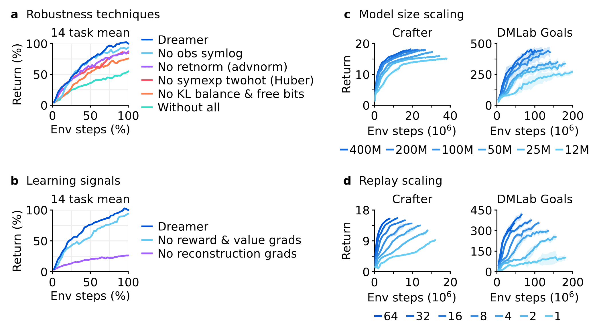
Moreover, in the ablation study, the authors noted that each individual robustness techniques contributes to the overall performance of Dreamer, albeit certain techniques may only impact specific tasks. Additionally, the scaling properties of DreamerV3 demonstrate its ability to learn robustly across varying model sizes and replay ratios, providing a predictable way for enhancing performance given computational resources.
References
[1] Hafner et al. “Learning Latent Dynamics for Planning from Pixels”, ICML 2019
[2] Hafner et al. “Dream to Control: Learning Behaviors by Latent Imagination”, ICLR 2020 (oral)
[3] Hafner et al. “Mastering Atari with Discrete World Models”, ICLR 2021
[4] Hafner et al. “Mastering Diverse Domains through World Models”, arXiv 2023
Leave a comment