
[RL] Distributional RL
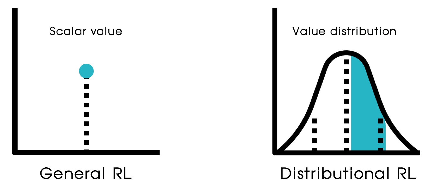
The ultimate goal of agent in RL is to maximize its cumulative reward obtained from interactions with an environment. An agent maximizes its return by making decisions that either yield immediate positive consequences or guide it into a desirable state. Thus, a particular assignment of reward to states and decisions directly affects the agent’s objective. To model this uncertainty, RL introduces an element of chance to the rewards (reward function \(r(\mathbf{s}_t, \mathbf{a}_t)\)) and the effects of the agent’s decisions (transition probability \(p(\mathbf{s}_{t+1} \vert \mathbf{s}_t, \mathbf{a}_t)\)) on its environment. Because the return is the sum of rewards received along the way, the general idea in RL, and this is fairly widely accepted, is to use the average of the possible outcomes as a measure of the value of a policy.
Distributional RL stems from the perspective that modeling the expected return alone fails to account for many complex phenomena that arise from interactions with the environment. Instead of the expectation, it considers return distribution; the probability of different returns that can be obtained as an agent interacts with its environment from a given state.
Therefore, extending from the general RL framework to the distributional framework involves generalizing scalar returns into random variables. For instance, the distribution Bellman equation of random return is derived from the Bellman equation of return as follows:
\[\begin{gathered} V^\pi (\mathbf{s}) = \mathbb{E}_{\pi} [r(\mathbf{s}_t, \mathbf{a}_t) + \gamma V^\pi (\mathbf{s}_{t+1}) \vert \mathbf{s}_t = \mathbf{s}] \\ \Downarrow \\ G^\pi (\mathbf{s}) \overset{\mathcal{D}}{=} R + \gamma G^\pi (\mathbf{s}^\prime) \end{gathered}\]where $G^\pi (\mathbf{s})$, $R$, $\mathbf{s}^\prime$, and $G^\pi (\mathbf{s}^\prime)$ are all random variables and $\overset{\mathcal{D}}{=}$ indicates equality between their distributions. However, several challenges arise from this seemingly simple change, such as measuring the quality of an agent’s predictions, determining optimality, and addressing computational complexities. We will also discuss these challenges in greater detail in subsequent sections and in the next post.
Preliminary: Bellman Operators
Let $V^\pi \in \mathbb{R}^\mathcal{S}$. To concisely express the Bellman equation, we define the following operator:
The Bellman operator is the mapping $\mathcal{T}^\pi: \mathbb{R}^\mathcal{S} \to \mathbb{R}^\mathcal{S}$ defined by $$ (\mathcal{T}^\pi V) (\mathbf{s}) = \mathbb{E}_\pi [r(\mathbf{s}_t, \mathbf{a}_t) + \gamma V (\mathbf{s}_{t+1}) \vert \mathbf{s}_t = \mathbf{s}] $$ where $V \in \mathbb{R}^\mathcal{S}$ is a value function estimate of $V^\pi$. For compact expression, the value estimate $V$ is often treated as finite-dimensional vector and the Bellman operator is also expressed in terms of vector operations: $$ \mathcal{T}^\pi V = r^\pi + \gamma \mathcal{P}^\pi V $$ where $r^\pi (\mathbf{s}) = \mathbb{E}_\pi [r(\mathbf{s}_t, \mathbf{a}_t) \vert \mathbf{s}_t = \mathbf{s}]$ and $\mathcal{P}^\pi$ is the transition operator defined as $$ (\mathcal{P}^\pi V) (\mathbf{s}) = \sum_{\mathbf{a} \in \mathcal{A}} \pi (\mathbf{a} \vert \mathbf{s}) \sum_{\mathbf{s}^\prime \in \mathcal{S}} \mathcal{P} (\mathbf{s}^\prime \vert \mathbf{s}, \mathbf{a}) V(\mathbf{s}^\prime) $$
Hence, the Bellman equation is simply reduced to $V = \mathcal{T}^\pi V$, and the true value function $V^\pi$ is the solution of the equation; that is, $V^\pi$ is the fixed point of the Bellman operator $\mathcal{T}^\pi$. And theoretically, it is known that $V^\pi$ is the unique solution of the Bellman equation, equivalently the unique fixed point of the Bellman operator, which can be demonstrated by contraction mapping.
An operator $F$ on a normed vector space $\mathcal{V}$ is a $\lambda$-contraction mapping with respect to norm $\Vert \cdot \Vert$ for $0 < \lambda < 1$ if $$ \Vert F (\mathbf{x}) - F (\mathbf{y}) \Vert \leq \lambda \Vert \mathbf{x} - \mathbf{y} \Vert $$ for all $\mathbf{x}, \mathbf{y} \in \mathcal{V}$. Intuitively, its application to different elements brings them closer by at least a constant multiplicative factor.
Then the following proposition holds:
The Bellman operator $\mathcal{T}^\pi$ is $\gamma$-contraction mapping with respect to $\Vert \cdot \Vert_\infty$: $$ \Vert \mathcal{T}^\pi V - \mathcal{T}^\pi V^\prime \Vert_\infty \leq \gamma \Vert V - V^\prime \Vert_\infty $$ for any two value functions $V, V^\prime \in \mathcal{R}^\chi$, where $\gamma$ is the discount factor.
$\color{#bf1100}{\mathbf{Proof.}}$
Recall the definition of infinity norm:
\[\Vert V \Vert_\infty = \underset{\mathbf{s} \in \mathcal{S}}{\max} \vert V(\mathbf{s}) \vert\]Hence, the following inequality is trivial:
\[\Vert \mathcal{P}^\pi V \Vert_\infty \leq \Vert V \Vert_\infty\]Then we have
\[\begin{aligned} \Vert \mathcal{T}^\pi V - \mathcal{T}^\pi V^\prime \Vert_\infty & = \Vert \gamma \mathcal{P}^\pi V - \gamma \mathcal{P}^\pi V^\prime \Vert_\infty \\ & = \gamma \Vert \mathcal{P}^\pi (V - V^\prime) \Vert_\infty \\ & \leq \gamma \Vert V - V^\prime \Vert_\infty \end{aligned}\] \[\tag*{$\blacksquare$}\]And Banach fixed-point theorem, also known as Banach-Caccioppoli theorem, guarantees the uniqueness of fixed point of a contraction mapping. Moreover, it ensures the convergence of consecutive applications of the Bellman operator to the fixed point; the true value estimate. This theorem theoretically underpins several computational methods, such as dynamic programming and TD learning.
Let $(\mathcal{V}, d)$ be complete metric space. For any $\lambda$-contraction mapping $\mathcal{T}: \mathcal{V} \to \mathcal{V}$, the followings hold:
- $\mathcal{T}$ admits an unique fixed point $\mathbf{v}^*$;
- for any given initial point $\mathbf{v}_0 \in \mathcal{V}$, the consecutive applications of $\mathcal{T}$ converges to $\mathbf{v}^*$: $$ \lim_{n \to \infty} \mathbf{v}_n = \mathbf{v}^* \text{ where } \mathbf{v}_n = \mathcal{T} (\mathbf{v}_{n-1}) $$ at a linear convergence rate determined by $\lambda$;
$\color{red}{\mathbf{Proof.}}$
For all $n \in \mathbb{N}$, the following inequality holds:
\[d(\mathbf{v}_{n+1}, \mathbf{v}_n) \leq \lambda^n d (\mathbf{v}_1, \mathbf{v}_0)\]Then, \(\{ \mathbf{v}_n \}_{n=1}^\infty\) is clearly Cauchy sequence:
$\color{black}{\mathbf{Proof.}}$
For any $m > n$:
\[\begin{aligned} d(\mathbf{v}_{m},\mathbf{v}_{n}) & \leq d(\mathbf{v}_{m},\mathbf{v}_{m-1}) + d(\mathbf{v}_{m-1}, \mathbf{v}_{m-2}) + \cdots + d(\mathbf{v}_{n+1},\mathbf{v}_{n}) \\ & \leq \lambda^{m-1} d(\mathbf{v}_{1},\mathbf{v}_{0}) + \lambda^{m-2} d(\mathbf{v}_{1}, \mathbf{v}_{0}) + \cdots + \lambda^{n}d(\mathbf{v}_{1}, \mathbf{v}_{0})\\ & = \lambda^{n} d(\mathbf{v}_{1},\mathbf{v}_{0}) \sum _{k=0}^{m-n-1} \lambda^{k}\\ & \leq \lambda^{n} d(\mathbf{v}_{1},\mathbf{v}_{0})\sum _{k=0}^{\infty }\lambda^{k} \\ & = \lambda^{n} d(\mathbf{v}_{1},\mathbf{v}_{0}) \left({\frac{1}{1-\lambda}}\right). \end{aligned}\]Let any $\varepsilon > 0$ be given. As $\lambda\ in [0, 1)$, there exists a large $N \in \mathcal{N}$ such that
\[\lambda^N < \frac{\varepsilon (1-\lambda)}{d(\mathbf{v}_1, \mathbf{v}_0)}\]Therefore, by choosing $m > n > N$:
\[d(\mathbf{v}_m, \mathbf{v}_n) < \varepsilon.\] \[\tag*{$\blacksquare$}\]By completeness of $(\mathcal{V}, d)$, the Cauchy sequence has a limit $\mathbf{v}^* \in \mathcal{V}$. Moreover, $\mathbf{v}^*$ must be a fixed point of $\mathcal{T}$:
\[\mathbf{v}^* = \lim_{n\to\infty} \mathbf{v}_n = \lim_{n\to\infty} \mathcal{T}(\mathbf{v}_{n-1}) = \mathcal{T} (\lim_{n\to\infty} \mathbf{v}_{n-1}) = \mathcal{T} (\mathbf{v}^*).\] \[\tag*{$\blacksquare$}\]Distributional Bellman Equation
Random Variable Bellman Equation
Consider a collection of random variables indexed by an initial state $\mathbf{s}$, each generated by a random trajectory \((\mathbf{S}_t, \mathbf{A}_t, R_t)_{t≥0}\):
\[\begin{aligned} & \mathbf{S}_0 \sim \xi_0 \\ & \mathbf{A}_t \vert \mathbf{S}_t \sim \pi (\cdot \vert \mathbf{S}_t) \\ & R_t \vert (\mathbf{S}_t, \mathbf{A}_t) \sim \mathbb{P}_{\mathcal{R}} (\cdot \vert \mathbf{S}_t, \mathbf{A}_t) \\ & \mathbf{S}_{t+1} \vert (\mathbf{S}_t, \mathbf{A}_t, R_t) \sim \mathbb{P}_{\mathcal{S}} (\cdot \vert \mathbf{S}_t, \mathbf{A}_t) \end{aligned}\]where $\xi_0$ is the initial state distribution and under the joint distribution of these random variables $\mathbb{P}_\pi(\cdot \vert \mathbf{S}_0 = \mathbf{s})$. Then, recall that the definition of return is a discounted sum of random rewards:
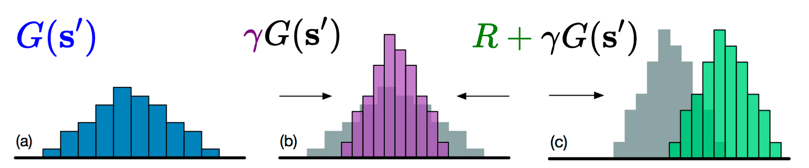
\[G = \sum_{t=0}^\infty \gamma^t R_t\]Now, as with value functions, to relate the return from the initial state to the random returns that occur downstream in the trajectory, define return-variable function as follows:
\[G^\pi (\mathbf{s}) = \sum_{t=0}^\infty \gamma^t R_t \text{ where } \mathbf{S}_0 = \mathbf{s}\]Note that $G^\pi (\mathbf{s})$ is defined as the random variable. And we can connect the value function $V^\pi$ of classical RL and $G^\pi$ as follows:
\[V^\pi (\mathbf{s}) = \mathbb{E}_\pi [G^\pi (\mathbf{s})]\]In case of random variable, we can show that the following Bellman equation holds in terms of equality in distribution instead of directly equating random variables.
Let $G^\pi$ be the return-variable function of policy $\pi$. For a sample transition $(\mathbf{S} = \mathbf{s}, \mathbf{A}, R, \mathbf{S}^\prime)$ independent of $G^\pi$, it holds that for any state $\mathbf{s} \in \mathcal{S}$, $$ G^\pi (\mathbf{s}) \overset{\mathcal{D}}{=} R + \gamma G^\pi (\mathbf{S}^\prime), \mathbf{S} = \mathbf{s} $$
$\color{red}{\mathbf{Proof.}}$
Consider the partial random return
\[G_{k: \infty} = \sum_{t=k}^\infty \gamma^{t- k} R_t \quad (k \in \mathbb{N})\]Note that $G^\pi (\mathbf{s}) \overset{\mathcal{D}}{=} G_{0: \infty}$ under the distribution $\mathbb{P}_\pi (\cdot \vert \mathbf{S}_0 = \mathbf{s})$. Then
\[\begin{aligned} G_{0: \infty} & = R_0 + \gamma G_{1: \infty} \\ & = R_0 + \gamma \sum_{\mathbf{s}^\prime \in \mathcal{S}} \mathbf{1} \{ \mathbf{S}_1 = \mathbf{s}^\prime \} G_{1:\infty} \end{aligned}\]By the Markov property, on the event that \(\mathbf{S}_1 = \mathbf{s}^\prime\), the return obtained from that point on is independent of the reward $R_0$. Furthermore, by the time-homogeneity property, on the same event, the return $G_{1:\infty}$ is equal in distribution to the return obtained when the episode begins at state $\mathbf{s}^\prime$. Therefore,
\[R_0 + \gamma \sum_{\mathbf{s}^\prime \in \mathcal{S}} \mathbf{1} \{ \mathbf{S}_1 = \mathbf{s}^\prime \} G_{1:\infty} \overset{\mathcal{D}}{=} R_0 + \gamma \sum_{\mathbf{s}^\prime \in \mathcal{S}} \mathbf{1} \{ \mathbf{S}_1 = \mathbf{s}^\prime \} G^\pi (\mathbf{s}^\prime) = R_0 + \gamma G^\pi (\mathbf{S}_1)\]and hence
\[G^\pi (\mathbf{s}) \overset{\mathcal{D}}{=} R_0 + \gamma G^\pi (\mathbf{S}_1)\] \[\tag*{$\blacksquare$}\]As a remark, the random-variable Bellman equation trivially implies the standard Bellman equation due to equality in distribution between the sample transition model $(\mathbf{S} = \mathbf{s}, \mathbf{A}, R, \mathbf{S}^\prime)$:
\[\begin{gathered} G^\pi(\mathbf{s}) \overset{\mathcal{D}}{=} R+\gamma G^\pi\left(\mathbf{S}^{\prime}\right) \\ \Longrightarrow \mathcal{D}_\pi\left(G^\pi(\mathbf{s})\right)=\mathcal{D}_\pi\left(R+\gamma G^\pi\left(\mathbf{S}^{\prime}\right) \mid \mathbf{S}=\mathbf{s}\right) \\ \Longrightarrow \mathbb{E}_\pi\left[G^\pi(\mathbf{s})\right]=\mathbb{E}_\pi\left[R+\gamma G^\pi\left(\mathbf{S}^{\prime}\right) \mid \mathbf{S}=\mathbf{s}\right] \\ \Longrightarrow V^\pi(\mathbf{s})=\mathbb{E}_\pi\left[R+\gamma V^\pi\left(\mathbf{S}^{\prime}\right) \mid \mathbf{S}=\mathbf{s}\right] \end{gathered}\]where $\mathcal{D} (Z) (A)$ denote the probability distribution of a random variable $Z$, $\mathbb{P} (Z \in A)$, and \(\mathcal{D}_\pi\) is the distribution of random variables derived from the joint distribution $\mathbb{P}_\pi$.
Distributional Bellman Equation
The random-variable Bellman equation is somewhat incomplete: it characterizes the distribution of the random return $G^\pi(\mathbf{s})$, but not the random variable itself. To eliminate the return-variable function $G^\pi$ and directly relate the distribution of the random return across different states, the distributional Bellman equation is introduced.
For given real-valued random variable $Z$ on probability space $(\Omega, \mathcal{F}, \mathbb{P})$ with probability distribution $\nu \in \mathscr{P}(\mathbb{R})$, recall the notation
\[\nu (S) = \mathbb{P} (Z \in S) \text { where } S \subseteq \mathbb{R}\]Denote the distribution of $G^\pi (\mathbf{s})$ by $\eta^\pi (\mathbf{s})$, which is called return-distribution function resulting in
\[\eta^\pi (\mathbf{s}) (A) = \mathbb{P} (G^\pi (\mathbf{s}) \in A) = \mathbb{P} (G^\pi (\mathbf{S}) \in A \vert \mathbf{S} = \mathbf{s}) \text { where } A \subseteq \mathbb{R}\]To construct the Bellman equation for return-distribution functions, consider the following operations over the space of probability distributions, which are analogous to the indexing into $G^\pi$, scaling by $\gamma$, and addition of $R$ in random-variable case:
- Mixing
Let us first consider the distribution of $G^\pi (\mathbf{S}^\prime)$: $$ \begin{aligned} \mathbb{P}_\pi (G^\pi (\mathbf{S}^\prime) \in A \vert \mathbf{S} = \mathbf{s}) & = \sum_{\mathbf{s}^\prime \in \mathcal{S}} \mathbb{P}_\pi (\mathbf{S}^\prime = \mathbf{s}^\prime \vert \mathbf{S} = \mathbf{s}) \mathbb{P}_\pi (G^\pi (\mathbf{s}^\prime) \in A) \\ & = \left( \sum_{\mathbf{s}^\prime \in \mathcal{S}} \mathbb{P}_\pi (\mathbf{S}^\prime = \mathbf{s}^\prime \vert \mathbf{S} = \mathbf{s}) \eta^\pi (\mathbf{s}^\prime) \right) (A) \\ \end{aligned} $$ That is, the probability distribution of $G^\pi (\mathbf{S}^\prime)$ is the mixture of $\eta^\pi$: $$ \begin{aligned} \mathcal{D}_\pi (G^\pi (\mathbf{S}^\prime) \vert \mathbf{S} = \mathbf{s}) & = \sum_{\mathbf{s}^\prime \in \mathcal{S}} \mathbb{P}_\pi (\mathbf{S}^\prime = \mathbf{s}^\prime \vert \mathbf{S} = \mathbf{s}) \eta^\pi (\mathbf{s}^\prime) \\ & = \mathbb{E}_\pi [\eta^\pi (\mathbf{S}^\prime) \vert \mathbf{S} = \mathbf{s}] \end{aligned} $$ - Scaling and Translation
To delineate the distribution of $R + \gamma G^\pi (\mathbf{S}^\prime)$, the notion of pushforward measure is introduced: $$ f_* (\nu) := \nu \circ f^{-1} = \mathcal{D}(f (Z)) $$ where $Z$ is the real-valued random variable with distribution $\nu$. Then, for two scalars $r \in \mathbb{R}$ and $\gamma \in [0, 1)$, define the bootstrap function $b_{r, \gamma}$: $$ b_{r, \gamma}: x \mapsto r + \gamma x $$ which leads to $$ (b_{r, \gamma})_* (\eta^\pi (\mathbf{S}^\prime)) = \mathcal{D}(r + \gamma G^\pi (\mathbf{S}^\prime)) $$
Observe that the push-forward is a linear operator from the trivial fact that the composition is linear transformation. This facilitates the combination of mixing, scaling, and translation of distribution, resulting in the distributional Bellman equation:
Let $\eta^\pi$ be the return-distribution function of policy $\pi$. For any state $\mathbf{s} \in \mathcal{S}$, we have $$ \eta^\pi (\mathbf{s}) = \mathbb{E}_\pi [(b_{R, \gamma})_* (\eta^\pi (\mathbf{S}^\prime)) \vert \mathbf{S} = \mathbf{s}] $$
$\color{red}{\mathbf{Proof.}}$
Let $B \subseteq \mathbb{R}$ and fix $\mathbf{s} \in \mathcal{S}$. Then, by the law of total expectation:
\[\begin{aligned} & \mathbb{P}_\pi (R + \gamma G^\pi (\mathbf{S}^\prime) \in B \vert \mathbf{S} = \mathbf{s}) \\ = & \sum_{\mathbf{a} \in \mathcal{A}} \pi (\mathbf{a} \vert \mathbf{s}) \sum_{\mathbf{s}^\prime \in \mathcal{S}} \mathbb{P}_{\mathcal{S}} (\mathbf{s}^\prime \vert \mathbf{s}, \mathbf{a}) \mathbb{P}_\pi (R + \gamma G^\pi (\mathbf{S}^\prime) \in B \vert \mathbf{S} = \mathbf{s}, \mathbf{A} = \mathbf{a}, \mathbf{S}^\prime = \mathbf{s}^\prime) \\ = & \sum_{\mathbf{a} \in \mathcal{A}} \pi (\mathbf{a} \vert \mathbf{s}) \sum_{\mathbf{s}^\prime \in \mathcal{S}} \mathbb{P}_{\mathcal{S}} (\mathbf{s}^\prime \vert \mathbf{s}, \mathbf{a}) \times \\ & \quad \mathbb{E}_{R \sim \mathbb{P}_{\mathcal{R}} (\cdot \vert \mathbf{s}, \mathbf{a})} [\mathbb{P}_\pi (R + \gamma G^\pi (\mathbf{s}^\prime) \in B \vert \mathbf{S} = \mathbf{s}, \mathbf{A} = \mathbf{a}, R) \vert \mathbf{S} = \mathbf{s}, \mathbf{A} = \mathbf{a} ] \\ = & \sum_{\mathbf{a} \in \mathcal{A}} \pi (\mathbf{a} \vert \mathbf{s}) \sum_{\mathbf{s}^\prime \in \mathcal{S}} \mathbb{P}_{\mathcal{S}} (\mathbf{s}^\prime \vert \mathbf{s}, \mathbf{a}) \mathbb{E}_{R \sim \mathbb{P}_{\mathcal{R}} (\cdot \vert \mathbf{s}, \mathbf{a})} [((b_{R, \gamma})_* (\eta^\pi (\mathbf{s}^\prime))) (B) \vert \mathbf{S} = \mathbf{s}, \mathbf{A} = \mathbf{a} ] \\ = & \mathbb{E}_\pi [((b_{R, \gamma})_* (\eta^\pi (\mathbf{S}^\prime))) (B) \vert \mathbf{S} = \mathbf{s}] \\ = & \mathbb{E}_\pi [((b_{R, \gamma})_* (\eta^\pi (\mathbf{S}^\prime))) \vert \mathbf{S} = \mathbf{s}] (B) \end{aligned}\]By the linearity of push-forward:
\[\begin{aligned} \mathcal{D}_\pi (R + \gamma G^\pi (\mathbf{S}^\prime) \vert \mathbf{S} = \mathbf{s} ) & = (b_{R, \gamma})_* (\mathcal{D}_\pi (G^\pi (\mathbf{S}^\prime) \vert \mathbf{S} = \mathbf{s})) \\ & = (b_{R, \gamma})_* (\mathbb{E}_\pi [\eta^\pi (\mathbf{S}^\prime) \vert \mathbf{S} = \mathbf{s}]) \\ & = \mathbb{E}_\pi [(b_{R, \gamma})_* (\eta^\pi (\mathbf{S}^\prime)) \vert \mathbf{S} = \mathbf{s}] \end{aligned}\]and the random-variable Bellman equation $G^\pi (\mathbf{s}) \overset{\mathcal{D}}{=} R + \gamma G^\pi (\mathbf{S}^\prime)$, the proof is completed.
\[\tag*{$\blacksquare$}\]Distributional Bellman Operator
Now, we can extend the notion of Bellman operator into distributional RL:
The random-variable Bellman operator is defined by the mapping from return-variable function (random variable) to another return-variable function: $$ (\mathcal{T}^\pi G)(\mathbf{s}) \overset{\mathcal{D}}{=} R (\mathbf{s}, \mathbf{a}) + \gamma G(\mathbf{S}^\prime), \mathbf{S} = \mathbf{s} $$ where $G(\mathbf{s}^\prime)$ is the indexing of the collection of random variables $G$ by $\mathbf{s}^\prime$.
The reason we use the same notation for two operations is due to the equivalence between the two operators, followed by the definition of distributional Bellman operator:
Given a probability distribution $\nu \in \mathscr{P}(\mathbb{R})$, a random variable $Z$ is called an instantiation of $\nu$ if $Z \sim \nu$. A collection of random variables $$G = \{G (\mathbf{s}): \mathbf{s} \in \mathcal{S} \}$$ is called an instantiation of $\nu$ if $\eta (\mathbf{S} = \mathbf{s}) = \mathcal{D} (\mathbf{G}(\mathbf{s})) \sim \nu$ for every $\mathbf{s} \in \mathcal{S}$.
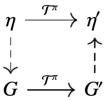
Let $\eta \in \mathscr{P}(\mathbb{R})^\mathcal{S}$, and let $G$ be an instantiation of $\eta$; $F_G = F_\eta$. For each $\mathbf{s} \in \mathcal{S}$, let $(\mathbf{S} = \mathbf{s}, \mathbf{A}, R, \mathbf{S}^\prime)$ be a sample transition independent of $G$. Then: $$ \mathcal{D}_\pi (R + \gamma G(\mathbf{S}^\prime) \vert \mathbf{S} = \mathbf{s}) = (\mathcal{T}^\pi \eta) (\mathbf{s}) $$
$\color{#bf1100}{\mathbf{Proof.}}$
First, the indexing transformation gives
\[\begin{aligned} \mathcal{D}_\pi (G(\mathbf{S}^\prime \vert \mathbf{S} = \mathbf{s})) & = \sum_{\mathbf{s}^\prime \in \mathcal{S}} \mathbb{P}_\pi (\mathbf{S}^\prime = \mathbf{s}^\prime \vert \mathbf{S} = \mathbf{s}) \eta (\mathbf{s}^\prime) \\ & = \mathbb{E}_\pi [\eta (\mathbf{S}^\prime) \vert \mathbf{S} = \mathbf{s}] \end{aligned}\]Next, scaling by $\gamma$ and adding the immediate reward $R$ yields
\[\mathcal{D}_\pi (R + \gamma G(\mathbf{S}^\prime) \vert \mathbf{S} = \mathbf{s}) = \mathbb{E}[ (b_{R, \gamma})_* (\eta (\mathbf{S}^\prime)) \vert \mathbf{S} = \mathbf{s} ].\] \[\tag*{$\blacksquare$}\]Then, we can formally express the fact that the return-distribution function $\eta^\pi$ is the only solution to the equation $\eta = \mathcal{T}^\pi \eta$, i.e. unique fixed point of $\mathcal{T}^\pi$.
$\color{red}{\mathbf{Proof.}}$
See Chapter 4.8. of Bellemare et al. 2023 for the proof;
\[\tag*{$\blacksquare$}\]Probabilistic Metrics
The theorem above can be proved using the notion of weak convergence, albeit at the cost of losing the convergence rate provided by the contractive mapping in the standard Bellman operator. This need for stronger guarantees motivates the development of contraction mapping theory with probability metrics that measure distances between distributions.
Contractivity
There are sufficient conditions for contractivity that a probability metric must satisfy. In this section, we first analyze the general behavior of the sequence of return function estimates with probability metrics.
Suppose that a probability metric $d$ is given: $$ d: \mathscr{P}(\mathbb{R}) \times \mathscr{P}(\mathbb{R}) \to [0, \infty] $$ To measure distances between return-distribution functions $\eta$ and $\eta^\prime$ that map an individual state to its probability distribution, we extend the probability metrics by considering the largest distance between probability distributions at individual states: $$ \bar{d}(\eta, \eta^\prime) = \underset{\mathbf{s} \in \mathcal{S}}{\sup} d(\eta (\mathbf{s}), \eta^\prime (\mathbf{s})) $$
Then, the following properties are required for $d$ to be sufficient conditions (but not necessary) for contractivity of $\bar{d}$. Observe that these properties are closely related to translation and scaling of random variable.
Let $p > 0$. The probability metric $d$ is $p$-homogeneous if for any scalar $\lambda \in [0, 1)$ and any two distributions $\mu, \nu \in \mathscr{P}(\mathbb{R})$ with associated random variables $X$, $Y$, we have $$ d (\lambda X, \lambda Y) = \lambda^p d(X, Y) $$ If no such $p$ exists, $d$ is referred to as inhomogeneous
The probability metric $d$ is regular if for any two distributions $\mu, \nu \in \mathscr{P}(\mathbb{R})$ with associated random variables $X$, $Y$, and an independent random variable $Z$, we have $$ d (X + Z, Y + Z) \leq d(X, Y) $$
Given $p \in [1, \infty)$, the probability metric $d$ is $p$-convex if for any $\lambda \in (0, 1)$ and two distributions $\mu_1$, $\mu_2$, $\nu_1$, $\nu_2 \in \mathscr{P}(\mathbb{R})$ with associated random variables $X_1$, $X_2$, $Y_1$, $Y_2$, respectively, we have $$ d^p (\lambda X_1 + (1 - \lambda) X_2, \lambda Y_1 + (1-\lambda) Y_2 ) \leq \lambda d^p (X_1, X_2) + (1-\lambda) d^p (Y_1, Y_2) $$ Note that this also implies an analogous property for mixtures of finitely many distributions.
Then, the following theorem holds:
Let $d$ be a given probability metric that is regular, $c$-homogeneous for some $c > 0$, and there exists $p \in [1, \infty)$ such that $d$ is $p$-convex. Then, for all return-distribution functions $\eta, \eta^\prime \in \mathscr{P}(\mathbb{R})^\mathcal{S}$, we have $$ \overline{d} (\mathcal{T}^\pi \eta, \mathcal{T}^\pi) \leq \gamma^c \overline{d}(\eta, \eta^\prime) $$ That is, the distributional Bellman operator $\mathcal{T}^\pi$ is $\gamma^c$-contractive mapping with respect to $\bar{d}$.
$\color{red}{\mathbf{Proof.}}$
Fix a state $\mathbf{s} \in \mathcal{S}$ and action $\mathbf{a} \in \mathcal{A}$, and consider the sample transition $(\mathbf{s}, \mathbf{a}, R, \mathbf{S}^\prime)$. Assume that $R$ and $\mathbf{S}^\prime$ are independent given $\mathbf{S}$ and $\mathbf{A}$:
\[R \sim \mathbb{P}_\mathcal{R} (\cdot \vert \mathbf{S}, \mathbf{A}) \quad \mathbf{S}^\prime \sim \mathbb{P}_\mathcal{S} (\cdot \vert \mathbf{S}, \mathbf{A})\]Let $G$ and $G^\prime$ be instantiations of $\eta$ and $\eta^\prime$, respectively. Define the state-action distributional Bellman operator $\mathcal{T}: \mathscr{P}(\mathbb{R})^\mathcal{S} \to \mathscr{P}(\mathbb{R})^{\mathcal{S} \times \mathcal{A}}$ given by
\[(\mathcal{T} \eta) (\mathbf{s}, \mathbf{a}) = \mathbb{E}[ (b_{R, \gamma})_* (\eta) (\mathbf{S}^\prime) \vert \mathbf{S} = \mathbf{s}, \mathbf{A} = \mathbf{a}]\]Note that $\mathcal{T}$ is defined independently of the policy $\pi$, since the action $\mathbf{a}$ is specified as an argument. Then,
\[\begin{aligned} d^p ((\mathcal{T} \eta) (\mathbf{s}, \mathbf{a}), (\mathcal{T} \eta^\prime) (\mathbf{s}, \mathbf{a})) & = d^p (R + \gamma G (\mathbf{S}^\prime), R + \gamma G^\prime (\mathbf{S}^\prime)) \\ & \leq d^p (\gamma G(\mathbf{S}^\prime), \gamma G^\prime (\mathbf{S}^\prime)) \quad \because \text{ regularity } \\ & = \gamma^{pq} d^p (G(\mathbf{S}^\prime), G^\prime(\mathbf{S}^\prime)) \quad \because q\text{-homogeneity } \\ & \leq \gamma^{pc} \sum_{\mathbf{s}^\prime \mathcal{S}} \mathbb{P}_\pi (\mathbf{S}^\prime = \mathbf{s}^\prime \vert \mathbf{S} = \mathbf{s}, \mathbf{A} = \mathbf{a}) d^p (G(\mathbf{s}^\prime), G^\prime (\mathbf{s}^\prime)) \quad \because p\text{-convexity } \\ & \leq \gamma^{pc} \underset{\mathbf{s}^\prime \in \mathcal{S}}{\sup} d^p (G(\mathbf{s}^\prime), G^\prime (\mathbf{s}^\prime)) \\ & = \gamma^{pc} \overline{d}^p (\eta, \eta^\prime) \end{aligned}\]Also, note that
\[(\mathcal{T}^\pi \eta) (\mathbf{s}) = \sum_{\mathbf{a} \in \mathcal{A}} \pi (\mathbf{a} \vert \mathbf{s}) (\mathcal{T} \eta) (\mathbf{s}, \mathbf{a})\]and hence by $p$-convexity of $d$:
\[\begin{aligned} d^p ( (\mathcal{T}^\pi \eta)(\mathbf{s}), (\mathcal{T}^\pi \eta^\prime) (\mathbf{s}) ) & \leq \pi (\mathbf{a} \vert \mathbf{s}) d^p ( (\mathcal{T}\eta) (\mathbf{s}, \mathbf{a}), (\mathcal{T}\eta^\prime) (\mathbf{s}, \mathbf{a}) ) \\ & = \gamma^{pq} \overline{d}^p (\eta, \eta^\prime) \end{aligned}\]Taking the supremum over $\mathbf{s} \in \mathcal{S}$ on the LHS and taking $p$-th roots then proves the result.
\[\tag*{$\blacksquare$}\]This demonstrates how the contractivity of the distributional Bellman operator $\mathcal{T}^\pi$ within the probability metric $d$ (specifically, in its supremum extension) arises from the inherent properties of $d$. For instace, we observed that the contraction modulus is intrinsically linked to the homogeneity of $d$, which, informally, denotes the degree to which scaling random variables by a factor $\gamma$ brings them “closer together”. And this theorem allows us to establish contractivity under various probability metrics, such as $\ell_p$ distances, which we will elaborate on.
However, in general, this theorem is insufficient to guarantee the convergence to $\eta^\pi$ due to the possibility of infinite distance, which harm the monotone convergence theorem. To formulate the additional condition for the convergence, the notion of finite domain is introduced:
For given probability metric $d$, its finite domain $\mathscr{P}_d (\mathbb{R}) \subseteq \mathscr{P} (\mathbb{R})$ is the set of probability distributions with finite first moment and finite $d$-distance to the zero-centered Dirac delta distribution: $$ \mathscr{P}_d (\mathbb{R}) = \{ \nu \in \mathscr{\mathbb{R}} \vert d(\nu, \delta_0) < \infty \text{ and } \mathbb{E}_{Z \sim \nu} [\vert Z \vert] < \infty \} $$ where $\delta_0$ is the instantiation of zero-centered Dirac delta distribution. The reference point (in this definition, $\delta_0$) can be any arbitrary fixed distribution.
Note that by the triangle inequality, for any $\mu, \nu \in \mathscr{P}_d (\mathbb{R})$, $d (\mu, \nu) < \infty$ is guaranteed. Then, the following convergence theorem holds:
Let $d$ be a probability metric with finite domain $\mathscr{P}_d (\mathbb{R})$ where the distributional Bellman operator $\mathcal{T}^\pi$ is contraction mapping with respect to $\bar{d}$. Suppose that
- $\eta^\pi \in \mathscr{P}_d (\mathbb{R})$
- $\mathscr{P}_d (\mathbb{R})$ is closed under $\mathcal{T}^\pi$; that is, $\forall \eta \in \mathscr{P}_d (\mathbb{R})^\mathcal{S}: \mathcal{T}^\pi \eta \in \mathscr{P}_d (\mathbb{R})^\mathcal{S}$
$\color{red}{\mathbf{Proof.}}$
Done by monotone convergence theorem.
\[\tag*{$\blacksquare$}\]Wasserstein Distance
One of the most well-known probability metrics is Wasserstein distance.
Let $\mu, \nu \in \mathscr{P}(\mathbb{R})$ be two probability distributions. A coupling between $\mu$ and $\nu$ is a joint distribution $\gamma \in \mathcal{P}(\mathbb{R}^2)$ such that if $(X, Y) \sim \gamma$ then also $X \sim \mu$ and $Y \sim \nu$.
Let $p \in [1, \infty)$. The $p$-Wasserstein distance between two distribution $\mu$ and $\nu$ is defined by $$ W_p (\mu, \nu) = \left( \underset{\gamma \in \prod (\mu, \nu)}{\inf} \mathbb{E}_{(X, Y) \sim \gamma} [\vert X - Y \vert^p] \right)^{1/p} $$ where $\prod (\mu, \nu) \subseteq \mathcal{P}(\mathbb{R}^2)$ is the set of all couplings of $\mu$ and $\nu$. The $\infty$-Wasserstein distance is defined by $$ W_\infty (\mu, \nu) = \underset{\gamma \in \prod (\mu, \nu)}{\inf} \mathbb{E}_{(X, Y) \sim \gamma} [\Vert X - Y \Vert_\infty (\gamma)] $$ where $$ \begin{aligned} \Vert X - Y \Vert_{\infty} (\gamma) & = \underset{m \in \mathbb{R}}{\inf} \left\{ \vert X - Y \vert \leq m \; \gamma\text{-a.e. for } (X, Y) \right\} \\ & = \underset{m \in \mathbb{R}}{\inf} \left\{ \mathbb{P}_{(X, Y) \sim \gamma} (\vert X - Y \vert > m) = 0 \right\} \end{aligned} $$
This enables the measurement of distance between two random variables $G(\mathbf{s})$ and $G(\mathbf{s}^\prime)$. Additionally, to measure distances between return-distribution functions that map an individual state to its probability distribution, we extend the Wasserstein distance by considering the largest Wasserstein distance between probability distributions at individual states:
Let $p \in [1, \infty)$. The supremum $p$-Wasserstein distance between two return-distribution $\eta_1$ and $\eta_2$ is defined by $$ \overline{W}_p (\mu, \nu) = \underset{\mathbf{s} \in \mathcal{S}}{\sup} W_p (\eta_1 (\mathbf{s}), \eta_2 (\mathbf{s})) $$
Based on these distances, the contractivity result regarding the distributional Bellman operator $\mathcal{T}^\pi$ can be derived:
The distributional Bellman operator $\mathcal{T}^\pi$ is $\gamma$-contraction mapping on $\mathscr{P}(\mathbb{R})^\mathcal{S}$ in the supremum $p$-Wasserstein distance $\overline{W}_p$ for all $p \in [1, \infty]$: $$ \overline{W}_p (\mathcal{T}^\pi \eta, \mathcal{T}^\pi \eta^\prime) \leq \gamma \overline{W}_p (\eta, \eta^\prime) $$
$\color{#bf1100}{\mathbf{Proof.}}$
Fix arbitrary $p \in [1, \infty)$. For each $\mathbf{s} \in \mathcal{S}$, consider the instantiation of $\eta (\mathbf{s})$ and $\eta^\prime (\mathbf{s})$ as the random variable $G(\mathbf{s})$ and $G^\prime(\mathbf{s})$, respectively. Let $(G(\mathbf{s})$, $G^\prime(\mathbf{s}))$ be the optimal coupling:
\[W_p ((\mathcal{T}^\pi \eta) (\mathbf{s}), (\mathcal{T}^\pi \eta^\prime) (\mathbf{s})) = \left( \mathbb{E}_{(X, Y) \sim \gamma} [\vert G(\mathbf{s}) - G(\mathbf{s}^\prime) \vert^p] \right)^{1/p}\]Consider the random transition $(\mathbf{s}, \mathbf{A}, R, \mathbf{S}^\prime)$ beginning in $\mathbf{s} \in \mathcal{S}$, constructed to be independent from $G$ and $G^\prime$. Write
\[\begin{aligned} \tilde{G}(\mathbf{s}) & = R + \gamma G(\mathbf{S}^\prime) \sim (\mathcal{T}^\pi \eta) (\mathbf{s}) \\ \tilde{G}^\prime(\mathbf{s}) & = R + \gamma G^\prime(\mathbf{S}^\prime) \sim (\mathcal{T}^\pi \eta^\prime) (\mathbf{s}) \end{aligned}\]Then
\[\begin{aligned} W_p^p ( (\mathcal{T}^\pi \eta) (\mathbf{s}), (\mathcal{T}^\pi \eta^\prime) (\mathbf{s}) ) & \leq \mathbb{E}_{\pi} \left[ \lvert \gamma G(\mathbf{S}^\prime) - \gamma G^\prime (\mathbf{S}^\prime) \rvert^p \vert \mathbf{S} = \mathbf{s} \right] \\ & = \gamma^p \sum_{\mathbf{s}^\prime \mathcal{S}} \mathbb{P}_\pi (\mathbf{S}^\prime = \mathbf{s}^\prime \vert \mathbf{S} = \mathbf{s}) \mathbb{E} \left[ \vert G(\mathbf{s}^\prime) - G^\prime (\mathbf{s}^\prime) \vert^p \right] \\ & = \gamma^p \underset{\mathbf{s}^\prime \in \mathcal{S}}{\sup} \mathbb{E} \left[ \vert G(\mathbf{s}^\prime) - G^\prime (\mathbf{s}^\prime) \vert^p \right] \\ & = \gamma^p \overline{W}_p^p ( \eta, \eta^\prime ) \end{aligned}\]The proof for $p = \infty$ is analagous to the above proof.
\[\tag*{$\blacksquare$}\]This proposition leads to the characterization of the convergence of the sequence $\eta_{k+1} = \mathcal{T}^\pi \eta_k$ to $\eta^\pi$:
Suppose that for each $(\mathbf{s}, \mathbf{a}) \in \mathcal{S} \times \mathcal{A}$, the reward distribution $\mathbb{P}_{\mathcal{R}} (\cdot \vert \mathbf{s}, \mathbf{a})$ is supported on the interval $[R_\min, R_\max]$. Then, for any initial return-distribution function $\eta_0$ whose distributions are bounded on the interval $[R_\min / (1-\gamma), R_\max / (1 - \gamma)]$, the sequence $\{ \eta_{k+1} = \mathcal{T}^\pi \eta_k \}_{k=0}^\infty$ converges to $\eta^\pi$ in the supremum $p$-Wasserstein distance for all $p \in [1, \infty]$: $$ \lim_{k \to \infty} \overline{W}_p (\eta_k, \eta^\pi) = 0 $$
$\color{red}{\mathbf{Proof.}}$
Denote by \(\mathscr{P}_B (\mathbb{R})\) the space of distributions bounded on $[V_\min = R_\min / (1-\gamma), V_\max = R_\max / (1-\gamma)]$. The following steps consequently show that for any initial \(\eta_0 \in \mathscr{P}_B (\mathbb{R})\), the sequence of iterates \(\{\eta_k\}_{k \geq 0}\) converges to $\eta^\pi$ by monotone convergence theorem. Note that bounded rewards guarantees the finite distance.
Step 1. $\eta^\pi \in \mathscr{P}_B (\mathbb{R})$
Since $R_t \in [R_\min, R_\max]$ for all $t$, for any state $\mathbf{s} \in \mathcal{S}$,
\[G^\pi (\mathbf{s}) = \sum_{t=0}^\infty \gamma^t R_t, \quad \mathbf{S}_0 = \mathbf{s}\]is guaranteed to be within $[V_\min, V_\max]$.
Step 2. $\mathcal{T}^\pi$ maps $\mathscr{P}_B (\mathbb{R})$ to $\mathscr{P}_B (\mathbb{R})$
Let $\eta \in \mathscr{P} (\mathbb{R})^\mathcal{S}$ and denote by $G$ an instantiation of $\eta$. For any $\mathbf{s} \in \mathcal{S}$,
\[\begin{aligned} \mathbb{P}_\pi (R + \gamma G(\mathbf{S}^\prime) \leq V_\max \vert \mathbf{S} = \mathbf{s}) & = \mathbb{P}_\pi (\gamma G(\mathbf{S}^\prime) \leq V_\max - R \vert \mathbf{S} = \mathbf{s}) \\ & \geq \mathbb{P}_\pi (\gamma G(\mathbf{S}^\prime) \leq V_\max - R_\max \vert \mathbf{S} = \mathbf{s}) \\ & = \mathbb{P}_\pi (G(\mathbf{S}^\prime) \leq V_\max \vert \mathbf{S} = \mathbf{s}) \\ & = 1. \end{aligned}\]Analogously,
\[\mathbb{P}_\pi (R + \gamma G(\mathbf{S}^\prime) \geq V_\min \vert \mathbf{S} = \mathbf{s}) = 1\]Since $R + \gamma G(\mathbf{S}^\prime), \mathbf{S} = \mathbf{s}$ is an instantiation of $(\mathcal{T}^\pi \eta)(\mathbf{s})$, we conclude that if $\eta \in \mathscr{P} (\mathbb{R})^\mathcal{S}$, then also $\mathcal{T}^\pi \eta \in \in \mathscr{P} (\mathbb{R})^\mathcal{S}$.
\[\tag*{$\blacksquare$}\]With the notion of finite domain, the condition of the above theorem can be generalized as follows:
$L_p$ metrics
There are also the family of probability metrics called $L_p$ metrics, the analogous concept of $L_p$ norm on $\mathbb{R}$.
Let $p \in [1, \infty)$. The distance $\ell_p: \mathscr{P}(\mathbb{R}) \times \mathscr{P}(\mathbb{R}) \to [0, \infty]$ is a probability metric defined by $$ \ell_p (\mu, \nu) = \left( \int_{\mathbb{R}} \vert F_\mu (x) - F_\nu (x) \vert^p \mathrm{d} x \right)^{1/p} $$ For $p = 2$, it is called Cramér Distance. For $p = \infty$, $\ell_\infty$, or Kolmogorov-Smirnov distance is defined by $$ \ell_\infty (\mu, \nu) = \underset{x \in \mathbb{R}}{\sup} \vert F_\mu (x) - F_\nu (x) \vert $$ For return-distribution functions $\eta, \eta^\prime \in \mathscr{P}(\mathbb{R})^\mathcal{S}$, the supremum $\ell_p$ are given by $$ \bar{\ell}_p (\eta, \eta^\prime) = \underset{\mathbf{s} \in \mathcal{S}}{\sup} \ell_p (\eta (\mathbf{s}), \eta^\prime (\mathbf{s})) $$
The distributional Bellman operator $\mathcal{T}^\pi$ is also a contraction mapping under the $\ell_p$ distances for $p \in [1, \infty)$ with a larger contraction modulus than $p$-Wasserstein distance:
For $p \in [1, \infty)$, the distributional Bellman operator $\mathcal{T}^\pi$ is $\gamma^{1/p}$-contraction mapping with respect to $\bar{\ell}_p$: $$ \bar{\ell}_p (\mathcal{T}^\pi \eta, \mathcal{T}^\pi \eta^\prime) \leq \gamma^{\frac{1}{p}} \bar{\ell}_p (\eta, \eta^\prime) $$ for all $\eta, \eta^\prime \in \mathscr{P}(\mathbb{R})^\mathcal{S}$. However, the contractivity doesn't hold for $\bar{\ell}_\infty$.
$\color{#bf1100}{\mathbf{Proof.}}$
It is sufficient to demonstrate that $\ell_p$ is $1/p$-homogeneous, regular, and $p$-convex.
$1/p$-homogeneity
Let $\mu, \nu \in \mathscr{P}(\mathbb{R})$ with associated random variable $X$, $Y$, respectively. Note that for $\lambda \in [0, 1)$:
\[F_{\lambda X} (x) F_X (\frac{x}{\lambda})\]We have
\[\begin{aligned} \ell_p^p (\lambda X, \lambda Y) & = \int_\mathbb{R} \lvert F_{\lambda X} (x) - F_{\lambda Y} (x) \rvert^p \mathrm{d} x \\ & = \int_\mathbb{R} \lvert F_{X} (\frac{x}{\lambda}) - F_{Y} (\frac{x}{\lambda}) \rvert^p \mathrm{d} x \\ & = \int_\mathbb{R} \lambda \lvert F_{X} (x) - F_{Y} (x) \rvert^p \mathrm{d} x \quad \because \text{ change of variable } \\ & = \gamma \ell_p^p (X, Y) \end{aligned}\]Regularity
Let $\mu, \nu \in \mathscr{P}(\mathbb{R})$, with independent instantiations of $\mu$ and $\nu$, $X$, $Y$, respectively, and let $Z$ be a random variable independent of $X$, $Y$. Then,
\[\begin{aligned} \ell_p^p\left(X + Z, Y + Z \right) & = \int_{\mathbb{R}} \lvert F_{X + Z}(x)-F_{Y + Z}(x) \rvert^p \mathrm{d} x \\ & =\int_{\mathbb{R}}\lvert \mathbb{E}_Z \left[F_X (x - Z)\right]-\mathbb{E}_Z \left[F_Y (x-Z)\right] \rvert^p \mathrm{d} x \\ & \leq \int_{\mathbb{R}} \mathbb{E}_W\left[\lvert F_X (x-Z) - F_Y (x- Z) \rvert^p\right] \mathrm{d} x \quad \because \text{Jensen's inequality} \\ & = \mathbb{E}_W \left[ \int_{\mathbb{R}}\lvert F_X (x-Z) - F_Y (x- Z) \rvert^p\right] \mathrm{d} x \quad \because \text{Fubini-Tonelli} \\ & = \ell_p^p \left(X, Y\right) \end{aligned}\]$p$-convexity
Let any $\lambda \in (0, 1)$ be given, and $\mu_1, \mu_2, \nu_1, \nu_2 \in \mathscr{P}(\mathbb{R})$. Note that
\[F_{\lambda \mu_1 + (1-\lambda) \mu_2} (x) = \lambda F_{\mu_1} (x) + (1-\lambda) F_{\mu_2} (x)\]By convexity of the mapping $x \mapsto \vert x \vert^p$ on $\mathbb{R}$ and Jensen’s inequality:
\[\begin{gathered} \vert F_{\lambda \mu_1 + (1-\lambda) \mu_2} (x) - F_{\lambda \nu_1 + (1-\lambda) \nu_2} (x) \vert^p \\ \leq \lambda \vert F_{\mu_1} (x) - F_{\mu_2} (x) \vert + (1 - \lambda) \vert F_{\nu_1} (x) - F_{\nu_2} (x) \vert^p \end{gathered}\]for all $x \in \mathbb{R}$. Thus
\[\ell_p^p (\lambda \mu_1 + (1 - \lambda) \mu_2, \lambda \nu_1 + (1 - \lambda) \nu_2) \leq \lambda \ell_p^p (\mu_1, \mu_2) + (1 - \lambda) \ell_p^p (\nu_1, \nu_2)\]$p = \infty$ case
However, note that the contractivity doesn’t hold for $\ell_\infty$. Consider a single-state process with zero reward, $\mathbb{P}_\mathcal{S} (\mathbf{S}^\prime = \mathbf{s} \vert \mathbf{S} = \mathbf{s}) = 1$ and $R = 0$ with $\gamma = 0.9$. Then, $\eta^pi (\mathbf{s})$ is a random variable $\delta_0$ that follows Dirac delta distribution centered at $0$. For counterexample, consider
\[\begin{aligned} \eta (\mathbf{s}) & = \delta_1 \\ \eta^\prime (\mathbf{s}) & = (\mathcal{T}^\pi \eta) (\mathbf{s}) = \delta_\gamma \end{aligned}\]Then, since for any $x \in (0, 1)$, thus
\[F_{\eta (\mathbf{s})} (x) = 0, F_{\eta^\pi (\mathbf{s})} (x) = 1 \implies \ell_\infty (\eta (\mathbf{s}), \eta^\pi (\mathbf{s})) = 1\]And the same argument with $x \in (0, \gamma)$ holds for $\eta^\prime$:
\[\ell_\infty (\eta^\prime (\mathbf{s}), \eta^\pi (\mathbf{s})) = 1\]Therefore, there is no $\lambda \in [0, 1)$ such that
\[\bar{\ell}_\infty (\eta^\prime, \eta^\pi) < \lambda \bar{\ell}_\infty (\eta, \eta^\pi)\] \[\tag*{$\blacksquare$}\]One way to relate it to our earlier result is to consider the behavior of the sequence defined by $\eta_{k+1} = \mathcal{T}^\pi \eta_k$. As measured in the $p$-Wasserstein distance, this sequence approaches $\eta^\pi$ at a rate of $\gamma$; but if we instead measure distances using the $\ell_p$ metric, this rate is slower, only $\gamma^{1/p}$. Don’t forget that the convergence is assure only within finite domain.
References
[1] Marc G. Bellemare and Will Dabney and Mark Rowland, “Distributional Reinforcement Learning”, MIT Press 2023
[2] Wikipedia, Banach fixed-point theorem
[3] Bellemare et al. “A Distributional Perspective on Reinforcement Learning”, ICML 2017
Leave a comment