
[RL] Distributional Dynamic Programming
Preliminary: Policy Evaluation
In classical reinforcement learning, the Bellman equation provides a simple equation for computing the value function $V^\pi$ of a policy $\pi$:
\[V^\pi = \mathcal{R}^\pi + \gamma \mathcal{P}^\pi V^\pi\]where $\mathcal{P}^\pi$ is the transition function and $\mathcal{R}^\pi$ is a vector
\[\mathcal{R}^\pi = \mathbb{E}_\pi [r(\mathbf{s}_t, \mathbf{a}_t) \vert \mathbf{s}_t = \mathbf{s}]\]By matrix algebra, we deduce that
\[V^\pi = (\mathbf{I} - \gamma \mathcal{P}^\pi)^{-1} \mathcal{R}^\pi\]When the matrix inversion is undesirable, the value function can instead be found by dynamic programming, particularly policy evaluation that successively computes
\[V_{k+1} = \mathcal{T}^\pi V_k \text{ where } (\mathcal{T}^\pi V) (\mathbf{s}) = \mathbb{E}_\pi [r(\mathbf{s}_t, \mathbf{a}_t) + \gamma V (\mathbf{s}_{t+1}) \vert \mathbf{s}_t = \mathbf{s}]\]Recall that the contractive nature of Bellman operator ensures the convergence of algorithm within finite number of iterations:
Let any initial value function estimate $V_0$ be given and construct a sequence by $$ V_{k+1} = \mathcal{T}^\pi V_k \text{ where } (\mathcal{T}^\pi V) (\mathbf{s}) = \mathbb{E}_\pi [r(\mathbf{s}_t, \mathbf{a}_t) + \gamma V (\mathbf{s}_{t+1}) \vert \mathbf{s}_t = \mathbf{s}] $$ For any $\varepsilon > 0$, if we set $K_\varepsilon$ by $$ K_\varepsilon \geq \frac{\log \varepsilon - \log \Vert V_0 - V^\pi \Vert_\infty}{\log \gamma} $$ then for all $k \geq K_\varepsilon$, we have $$ \Vert V_k - V^\pi \Vert_\infty \leq \varepsilon $$
$\color{red}{\mathbf{Proof.}}$
Recall that $\mathcal{T}^\pi$ is $\gamma$-contraction mapping with regard to $\Vert \cdot \Vert_\infty$ norm and $V^\pi$ is the unique fixed point by Banach fixed-point theorem. Then, for any $k \geq 1$:
\[\begin{aligned} \Vert V_k - V^\pi \Vert_\infty & = \Vert \mathcal{T}^\pi V_{k-1} - T^\pi V^\pi \Vert_\infty \\ & \leq \gamma \Vert V_{k-1} - V^\pi \Vert_\infty \\ & \leq \cdots \\ & \leq \gamma^k \Vert V_0 - V^\pi \Vert_\infty \end{aligned}\]By setting the RHS to be less than or equal to $\varepsilon$ and rearranging terms, done.
\[\tag*{$\blacksquare$}\]Distribution Parametrization
First, we denote by $\mathscr{F}$ the space of all possible return-distribution functions:
\[\mathscr{F} = \{ P_\theta \in \mathscr{P}(\mathbb{R}) \vert \theta \in \Theta \}\]Similar to policy evaluation, let’s consider an iterative algorithm that approximates the return-distribution function $\eta^\pi$ by repeatedly applying the distributional Bellman operator $\mathcal{T}^\pi$:
\[\eta_{k + 1} = \mathcal{T}^\pi \eta_k \text{ where } (\mathcal{T}^\pi \eta) (\mathbf{s}) = \mathbb{E}_{\pi} [ (b_{R, \gamma})_* (\eta) (\mathbf{S}^\prime) \vert \mathbf{S} = \mathbf{s}]\]From an algorithmic perspective, implementing this procedure necessitates the distributional Bellman operators that efficiently perform the shift-and-scale operation and compute mixtures of probability distributions. However, the nature of probability distributions are intractable and infinite-dimensional, thereby hindering the practical implementation of algorithm. Therefore, a first design decision for a general distributional RL algorithm is how probability distributions should be represented in an approximate way.
Empirical Representation
To avoid the computational costs associated with unbounded memory usage, we usually restrict probability distributions to be discrete described by a fixed number of parameters:
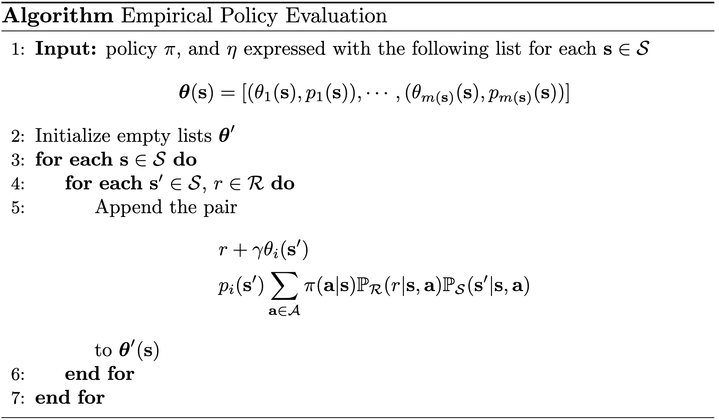
The empirical representation is the set $\mathscr{F}_E$ of empirical distributions: $$ \mathscr{F}_E = \left. \left\{ \sum_{i=1}^m p_i \delta_{\theta_i} \right\vert m \in \mathbb{N}, \theta_i \in \mathbb{R}, p_i \geq 0, \sum_{i=1}^m p_i = 1 \right\} $$ where $\delta_{\theta}$ is Dirac delta function centered at $\theta \in \mathbb{R}$. Therefore, an empirical distribution $\nu \in \mathscr{F}_E$ is represented as a finite list of pairs $(\theta_i, p_i)_{i=1}^m$. We call individual elements of such a distribution particles, each consisting of a probability and a location. In the context of return-distribution function $\eta (\mathbf{s})$, it can be written as $$ \eta (\mathbf{s}) = \sum_{i=1}^{m(\mathbf{s})} p_i (\mathbf{s}) \delta_{\theta_i (\mathbf{s})} $$
Consequently, the empirical representation of return-distribution function provides much convenient formulations for distributional Bellman operator:
- Push-forward measure
Let $\nu \in \mathscr{F}_E$ be an empirical distribution with parameters $m$ and $(\theta_i, p_i)_{i=1}^m$. For $r \in \mathbb{R}$ and $\gamma \in \mathbb{R}$: $$ (b_{r, \gamma})_* (\nu) = \sum_{i=1}^m p_i \delta_{r + \gamma \theta_i} $$ - Closedness of $\mathscr{F}_E$ under $\mathcal{T}^\pi$
If return-distribution function $\eta$ is an empirical distribution with parameters $\{ (p_i (\mathbf{s}), \theta_i (\mathbf{s}))_{i=1}^{m(\mathbf{s})} \vert \mathbf{s} \in \mathcal{S} \}$: $$ (\mathcal{T}^\pi \eta)(\mathbf{s})=\sum_{\mathbf{a} \in \mathcal{A}} \sum_{r \in \mathcal{R}} \sum_{\mathbf{s}^\prime \in \mathcal{S}} \mathbb{P}_\pi \left(\mathbf{A} = \mathbf{a}, R = r, \mathbf{S}^\prime = \mathbf{s}^\prime \vert \mathbf{S} = \mathbf{s} \right) \sum_{i=1}^{m(\mathbf{s}^\prime)} p_i (\mathbf{s}^\prime) \delta_{r + \gamma \theta_i (\mathbf{s}^\prime)} $$
$\color{#bf1100}{\mathbf{Proof.}}$
1. This statement is trivial by the definition of push-forward measure:
\[f_* (\mu) (A) = \mu \left( f^{-1} (A) \right)\]2. Fix state $\mathbf{s} \in \mathcal{S}$.
For brevity, denote by \(\mathbb{P}_\pi \left(\mathbf{A} = \mathbf{a}, R = r, \mathbf{S}^\prime = \mathbf{s}^\prime \vert \mathbf{S} = \mathbf{s} \right)\) $P_{\mathbf{a}, r, \mathbf{s}^\prime}$. Then we can show that $(\mathcal{T}^\pi \eta) (\mathbf{s})$ follows empirical distribution again from the first statement of proposition:
\[\begin{aligned} (\mathcal{T}^\pi \eta)(\mathbf{s}) & = \sum_{\mathbf{a} \in \mathcal{A}} \sum_{r \in \mathcal{R}} \sum_{\mathbf{s}^\prime \in \mathcal{S}} P_{\mathbf{a}, r, \mathbf{s}^\prime} (b_{r, \gamma})_* (\eta) (\mathbf{s}^\prime) \\ & = \sum_{\mathbf{a} \in \mathcal{A}} \sum_{r \in \mathcal{R}} \sum_{\mathbf{s}^\prime \in \mathcal{S}} P_{\mathbf{a}, r, \mathbf{s}^\prime} (b_{r, \gamma})_* \left( \sum_{i=1}^{m(\mathbf{s}^\prime)} p_i (\mathbf{s}^\prime) \delta_{\theta_i (\mathbf{s}^\prime)} \right) (\mathbf{s}^\prime) \\ & = \sum_{\mathbf{a} \in \mathcal{A}} \sum_{r \in \mathcal{R}} \sum_{\mathbf{s}^\prime \in \mathcal{S}} P_{\mathbf{a}, r, \mathbf{s}^\prime} \sum_{i=1}^{m(\mathbf{s}^\prime)} p_i (\mathbf{s}^\prime) \delta_{r + \gamma \theta_i (\mathbf{s}^\prime)} (\mathbf{s}^\prime) \\ & \equiv \sum_{j=1}^{m^\prime} p^{\prime}_j \delta_{\theta^{\prime}_j} \\ \end{aligned}\]for some collection \(({p^\prime}_j, \theta^{\prime}_j)_{j=1}^{m^\prime}\).
\[\tag*{$\blacksquare$}\]The empirical representation of the distribution space can alleviate the computational burden of the empirical policy evaluation. Furthermore, since $\mathscr{F}_E$ is closed under $\mathcal{T}^\pi$, we can examine the behavior of this procedure via the theory of contraction mappings. In particualr, we estabilish a bound on the number of iterations required to to achieve an $\varepsilon$-approximation of the return-distribution function $\eta^\pi$ with respect to Wasserstein distance in the next theorem.
Assume that the reward distributions $\mathbb{P}_\mathcal{R}( \cdot \vert \mathbf{s}, \mathbf{a})$ are supported on a finite set $\mathcal{R}$, thereby ensuring the existence of an interval $[V_\min, V_\max]$ within which the returns lie. Let $\eta_0 (\mathbf{s}) = \delta_0$ for all $\mathbf{s} \in \mathcal{S}$ be an initial return-distribution function and consider the iterative procedure that computes $$ \eta_{k+1} = \mathcal{T}^\pi \eta_k $$ For any $\varepsilon > 0$, if we set $K_\varepsilon$ by $$ K_\varepsilon \geq \frac{\log \varepsilon - \log (\max \{ \vert V_\min \vert , \vert V_\max \vert \})}{\log \gamma} $$ then for all $k \geq K_\varepsilon$, we have $$ \overline{W}_p (\eta_k, \eta^\pi) \leq \varepsilon \quad \forall p \in [1, \infty] $$ where $\overline{W}_p$ is the supremum $p$-Wasserstein distance.
$\color{red}{\mathbf{Proof.}}$
Since $\mathcal{T}^\pi$ is a contraction mapping with respect to $\overline{W}p$ and $\eta^\pi$ is its fixed point for the finite supported $\mathbb{P}\mathcal{R}$, the following holds:
\[\overline{W}_p (\eta_k, \eta^\pi) \leq \gamma^k \overline{W}_p (\eta_0, \eta^\pi)\]Since $\eta_0 = \delta_0$ and $\eta^\pi$ is supported on $[V_\min, V_\max]$, it is possible to upper-bound \(\overline{W}_p (\eta_0, \eta^\pi)$ by $\max (\vert V_\min \vert, \vert V_\max \vert)\). Setting the RHS to be less than or equal to $\varepsilon$ and rearranging gives the inequality for $K_\varepsilon$.
\[\tag*{$\blacksquare$}\]Fixed-size Empirical Representations
The empirical representation is expressive because it can use more particles to describe more complex probability distributions. However, such expansion leads to the algorithm intractability since the number of parameters that describe the return-distribution may grow exponentially in current length.
A desirable restriction is to fix the number and type of particles used to represent probability distributions, of which parametrizations are subsets of the empirical representation $\mathscr{F}_E$:
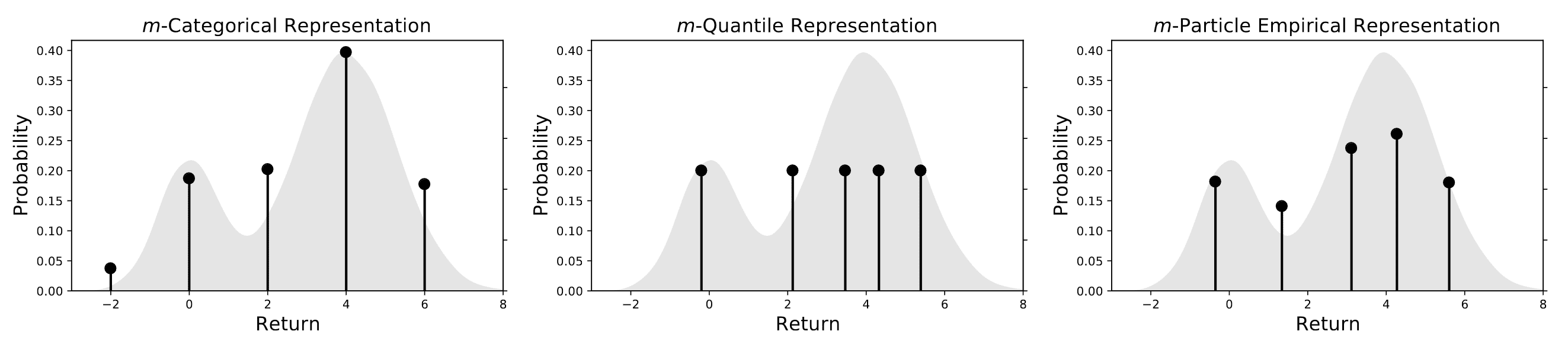
The $m$-particle representation is the set $\mathscr{F}_{E,m}$ of empirical distributions with fixed number $m$ of parameter pairs: $$ \mathscr{F}_{E, m} = \left. \left\{ \sum_{i=1}^m p_i \delta_{\theta_i} \right\vert \theta_i \in \mathbb{R}, p_i \geq 0, \sum_{i=1}^m p_i = 1 \right\} $$ where $\delta_{\theta}$ is Dirac delta function centered at $\theta \in \mathbb{R}$. Therefore, an empirical distribution $\nu \in \mathscr{F}_E$ is represented as a finite list of particles $(\theta_i, p_i)_{i=1}^m$ with $2m -1$ parameters.
Frequently, categorical and quantile representations are used for fixed-size empirical representations. By committing to either fixed locations or fixed probabilities, we can further simplifies algorithmic design.
The $m$-particle representation parameterizes the location of $m$ equally weighted particles: $$ \mathscr{F}_{Q, m} = \left. \left\{ \frac{1}{m} \sum_{i=1}^m \delta_{\theta_i} \right\vert \theta_i \in \mathbb{R} \right\} $$
Given a collection of m evenly spaced locations $\theta_1 < \cdots < \theta_m$, the $m$-categorical representation parameterizes the probability of $m$ particles at these fixed locations: $$ \mathscr{F}_{C, m} = \left. \left\{ \sum_{i=1}^m p_i \delta_{\theta_i} \right\vert p_i \geq 0, \sum_{i=1}^m p_i = 1 \right\} $$
Projection
Having computed $\mathcal{T}^\pi \eta_k$, the supports of this new distributions typically no longer lies in the parametric family $\mathcal{P}$; especially such closedness is not guaranteed on fixed-size empirical representations. To get around this issue, we necessitate projection operator:
\[\Pi_\mathscr{F}: \mathscr{P}(\mathbb{R}) \to \mathscr{F}\]that may be applied to each real-valued distribution in a return-distribution function to obtain the best achievable approximation within the target representation $\mathscr{F}$:
For given probability metric $d$, $d$-projection of $\nu \in \mathscr{P}(\mathbb{R})$ onto $\mathscr{F}$ is a function $\Pi_{\mathscr{F}, d}: \mathscr{P}(\mathbb{R}) \to \mathscr{F}$ that finds a distribution $\hat{\nu} \in \mathscr{F}$ $d$-closest to $\nu$: $$ \Pi_{\mathscr{F}, d} \nu \in \underset{\hat{\nu} \in \mathscr{F}}{\arg \min} \; d(\nu, \hat{\nu}) $$ Note that neither the existence nor uniqueness of a $d$-projection $\Pi_{\mathscr{F}, d}$ is actually guaranteed in most general cases.
Categorical Projection
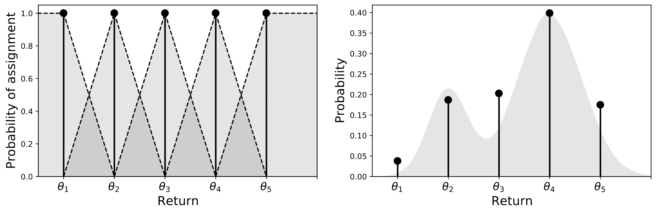
Bellemare et al. 2017 proposed the heuristic projection operator $\Pi_C$, assigning the probability mass $q$ of a particle located at $z$ to the two locations nearest to $z$ in the fixed support \(\{\theta_1, \cdots, \theta_m \}\). Specifically, the categorical projection of $\nu \in \mathscr{P}(\mathbb{R})$ takes the form
\[\Pi_C \nu = \sum_{i=1}^m p_i \delta_{\theta_i}\]where $\varsigma_i$ is the stride between successive particles and $p_i$ is defined by
\[p_i = \mathbb{E}_{Z \sim \nu} \left[h_i \left( \frac{Z - \theta_i}{\varsigma_i = \theta_{i+1} - \theta_{i}} \right) \right]\]for a set of triangle kernels $h_i: \mathbb{R} \to [0, 1]$ that converts the length to the probability:
\[\begin{aligned} h_1 (z) & = \begin{cases} 1 & \quad z \leq 0 \\ \max (0, 1 - \vert z \vert) & \quad z > 0 \end{cases} \\ h_2 (z) & = \cdots = h_{m-1} (z) = \max (0, 1 - \vert z \vert) \\ h_m (z) & = \begin{cases} \max (0, 1 - \vert z \vert) & \quad z \leq 0 \\ 1 & \quad z > 0 \end{cases} \end{aligned}\]Note that the parameters of the extreme locations are computed differently with half-triangular kernels, as these also encompass the probability mass associated with values exceeding $\theta_m$ and falling below $\theta_1$. Consequently, the triangular kernel can allocate probability mass from $\nu$ to the location $\theta_i$ in proportion to the distance to its adjacent point.
The following proposition justifies that such a parameterization of $p_i$ results in a valid $\ell_2$-projection of $\nu$.
Let $\nu \in \mathscr{P}(\mathbb{R})$. The projection $\Pi_C \nu$ is a unique $\ell_2$-projection of $\nu$ onto $\mathscr{F}_{C, m}$.
$\color{#bf1100}{\mathbf{Proof.}}$
In this proof, we demonstrate the following Pythagorean identity:
For any $\nu \in \mathscr{P}_{\ell_2} (\mathbb{R})$ and $\nu^\prime \in \mathscr{F}_{C, m}$, we have $$ \ell_2^2 (\nu, \nu^\prime) = \ell_2^2 (\nu, \Pi_C \nu) + \ell_2^2 (\Pi_c \nu, \nu^\prime) $$
$\color{black}{\mathbf{Proof.}}$
We first estabilish an intepretation of the CDF of $\Pi_C \nu$ as averaging CDF values of $\nu$ on each interval $(\theta_i, \theta_{i+1})$ for $i = 1, \cdots, m-1$. Note that for $z \in (\theta_i, \theta_{i+1}]$, we have
\[\begin{aligned} h_i (\frac{z - \theta_i}{\varsigma_i}) & = 1 - \frac{\vert z - \theta_i \vert}{\theta_{i+1} - \theta_i} \\ & = \frac{\theta_{i+1} - \theta_i + \theta_i - z}{\theta_{i+1} - \theta_i} \\ & = \frac{\theta_{i+1} - z}{\theta_{i+1} - \theta_i} \end{aligned}\]For $i = 1, \cdots, m - 1$, we have
\[\begin{aligned} F_{\Pi_C \nu} (\theta_i) & = \sum_{j=1}^i \mathbb{E}_{Z \sim \nu} [h_j (Z)] \\ & = \mathbb{E}_{Z \sim \nu} \left[ \mathbf{1} \{ Z \leq \theta_i\} + \mathbf{1} \{ Z \in (\theta_i, \theta_{i+1}] \} \frac{\theta_{i+1} - Z}{\theta_{i+1} - \theta_i} \right] \\ & = \frac{1}{\theta_{i+1} - \theta_i} \int_{\theta_i}^{\theta_{i+1}} F_\nu (z) \mathrm{~d}z. \end{aligned}\]Then, since $F_{\Pi_C \nu} = F_{\nu^\prime}$ on $(-\infty, \theta_1)$ and $(\theta_m, \infty)$, and on each interval $(\theta_i, \theta_{i+1})$, $F_{\Pi_C \nu} - F_{\nu^\prime}$ is constant and $F_{\Pi_C \nu}$ is constant and equals to average of $F_\nu$ on the interval:
\[\begin{gathered} \int_{\theta_i}^{\theta_{i+1}} (F_\nu (z) - F_{\Pi_C v}(z)) (F_{\Pi_C \nu}(z) - F_{\nu^\prime}(z)) \mathrm{d} z \\ = (F_{\Pi_C \nu}(z) - F_{\nu^\prime}(z)) \int_{\theta_i}^{\theta_{i+1}} (F_\nu (z) - F_{\Pi_C v}(z)) \mathrm{d} z = 0, \end{gathered}\]we have
\[\begin{aligned} & \ell_2^2 (\nu, \nu^\prime ) = \int_{-\infty}^{\infty} [F_\nu(z)-F_{\nu^\prime }(z)]^2 \mathrm{~d}z \\ & = \int_{-\infty}^{\infty} [F_\nu (z) - F_{\Pi_C \nu}(z)]^2 \mathrm{~d} z + \int_{-\infty}^{\infty}\left(F_{\Pi_C \nu}(z) - F_{\nu^\prime}(z)\right)^2 \mathrm{~d} z \\ & + 2 \int_{-\infty}^{\infty} (F_\nu (z) - F_{\Pi_C v}(z)) (F_{\Pi_C \nu}(z) - F_{\nu^\prime}(z)) \mathrm{d} z \\ & = \ell_2^2 (\nu, \Pi_C \nu) + \ell_2^2 (\Pi_C \nu, \nu^\prime) \\ & + 2\left(\int_{-\infty}^{\theta_1} + \sum_{i=1}^{m-1} \int_{\theta_i}^{\theta_{i+1}} + \int_{\theta_m}^{\infty}\right) (F_\nu(z)-F_{\Pi_C \nu}(z))(F_{\Pi_C \nu}(z) - F_{\nu^\prime }(z)) \mathrm{d} z \\ & = \ell_2^2 (\nu, \Pi_C \nu) + \ell_2^2 (\Pi_C \nu, \nu^\prime) \end{aligned}\] \[\tag*{$\blacksquare$}\]Then, it follows that $\nu^\prime = \Pi_C \nu$ is the unique $\ell_2$-projection of $\nu$ onto $\mathscr{F}_{C, m}$, since this choice of $\nu^\prime$ uniquely minimizes the RHS.
\[\tag*{$\blacksquare$}\]Quantile Projection
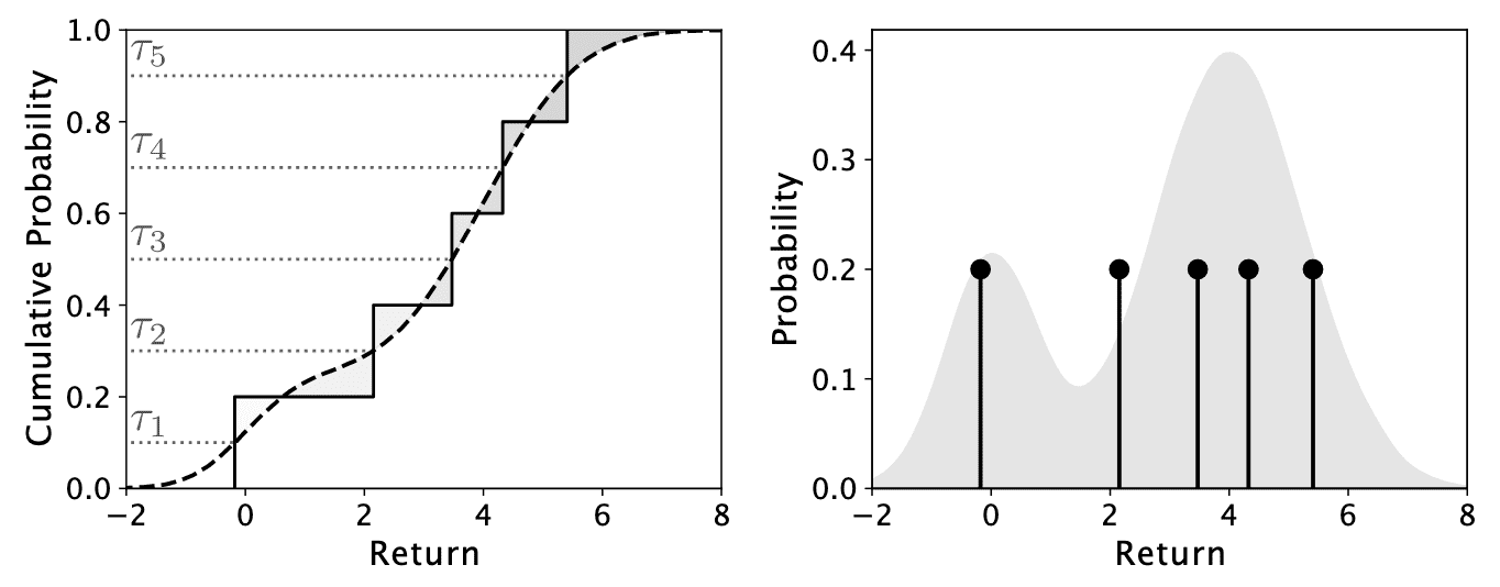
In case of quantile representation, the 1-Wasserstein distance $W_1$ can be expressed in closed form and is straightforward to implement. The quantile projection $\Pi_Q$ must take the form
\[\Pi_{Q} \nu = \frac{1}{m} \sum_{i=1}^m \delta_{\theta_i}\]For the parametrization of $\theta_i$, the following lemma offers insight: the $i$-th particle of a $m$-quantile distribution is “responsible” for the portion of the 1-Wasserstein distance measured on the interval $\left[ \frac{i-1}{m}, \frac{i}{m} \right]$.
Let $\nu \in \mathscr{P}(\mathbb{R})$ with CDF $F_\nu$. Let $0 \leq a < b \leq 1$. Then, a solution to the optimization problem: $$ \underset{\theta \in \mathbb{R}}{\min} \int_a^b \vert F_\nu^{-1} (\tau) - \theta \vert \mathrm{d} \tau $$ is given by the quantile midpoint $$ \theta = F_\nu^{-1} \left( \frac{a+b}{2} \right). $$
$\color{green}{\mathbf{Proof.}}$
To prove the statement, we need the notion of sub-gradient of the convex functions:
For a convex function $f: \mathbb{R} \to \mathbb{R}$, a sub-gradient $g : \mathbb{R} \to \mathbb{R}$ for $f$ is a function that satisfies $$ f (z_2) \geq f (z_1) + g(z_1)(z_2 − z_1). $$ for all $z_1, z_2 \in \mathbb{R}$.
Note that $\vert F_\nu^{-1}(\tau) - \theta \vert$ is convex function of $\tau$. And the sub-gradient for this function is given by
\[g_\tau (\theta) = \begin{cases} 1 & \quad \text{ if } \theta < F_\nu^{-1} (\tau) \\ -1 & \quad \text{ if } \theta > F_\nu^{-1} (\tau) \\ 0 & \quad \text{ if } \theta = F_\nu^{-1} (\tau) \\ \end{cases}\]A sub-gradient for our optimization problem is therefore
\[\begin{aligned} g_{[a, b]}(\theta) & = \int_{\tau=a}^b g_\tau(\theta) d \tau \\ & =\int_{\tau=a}^{F_v(\theta)}-1 \mathrm{~d} \tau+\int_{\tau = F_\nu(\theta)}^b 1 \mathrm{~d} \tau \\ & = - (F_\nu(\theta)-a) + (b-F_\nu(\theta)) \end{aligned}\]Setting the sub-gradient to zero and solving for $\theta$:
\[\begin{aligned} & 0 = a + b - 2F_\nu(\theta) \\ \implies & F_\nu(\theta) = \frac{a+b}{2} \\ \implies & \theta = F_\nu^{-1} \left( \frac{a+b}{2} \right) \end{aligned}\] \[\tag*{$\blacksquare$}\]Based on the lemma, the quantile midpoint $\frac{2i-1}{2m}$ minimizes the 1-Wasserstein distance to $\nu$ on the cumulative probability interval $\left[ \frac{i-1}{m}, \frac{i}{m} \right]$. The following proposition justifies that such a parameterization of $\theta_i$ results in a valid $W_1$-projection of $\nu$.
Let $\nu \in \mathscr{P}(\mathbb{R})$. The following projection $$ \Pi_{Q} \nu = \frac{1}{m} \sum_{i=1}^m \delta_{\theta_i} $$ where $$ \theta_i = F_\nu^{-1} \left( \frac{2i-1}{2m} \right) \quad i = 1, \cdots, m $$ is a $W_1$-projection of $\nu$ onto $\mathscr{F}_{Q, m}$.
$\color{#bf1100}{\mathbf{Proof.}}$
Let $\nu^\prime = \frac{1}{m} \sum_{i=1}^m \delta_{\theta_i}$ be a $m$-quantile distribution. Without loss of generality, assume that $\theta_1 \leq \cdots \theta_m$. For $\tau \in (0, 1)$, its inverse CDF is
\[F_{\nu^\prime}^{-1} (\tau) = \theta_{\lceil \tau m \rceil}.\]Observe thattThis function is constant on the intervals $(0, \frac{1}{m})$, $[\frac{1}{m}, \frac{2}{m})$, $\cdots$, $[\frac{m-1}{m}, 1)$. The 1-Wasserstein distance between $\nu$ and $\nu^{\prime}$ therefore decomposes into a sum of $m$ terms:
\[\begin{aligned} W_1 (\nu, \nu^\prime) & = \int_0^1 \vert F_\nu^{-1} (\tau) - F_{\nu^\prime}^{-1} (\tau) \vert \mathrm{~d} \tau \\ & = \sum_{i=1}^m \int_{\frac{(i-1)}{m}}^{\frac{i}{m}} \vert F_\nu^{-1} (\tau) - \theta_i \vert \mathrm{~d} \tau \end{aligned}\]From the previous lemma, we already know that the $i$-th term of the summation is minimized by the quantile midpoint:
\[F_\nu^{-1} (\frac{2i-1}{2m})\] \[\tag*{$\blacksquare$}\]Distributional Dynamic Programming
Embedding the projected Bellman operator in an for loop to obtain an algorithmic template for approximating the return-distribution function, we call such template distributional dynamic programming:
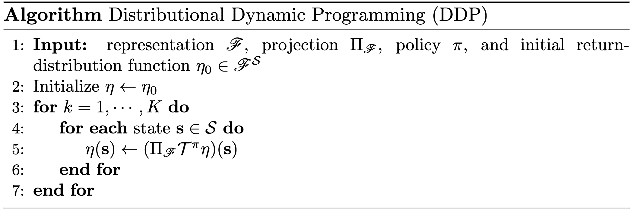
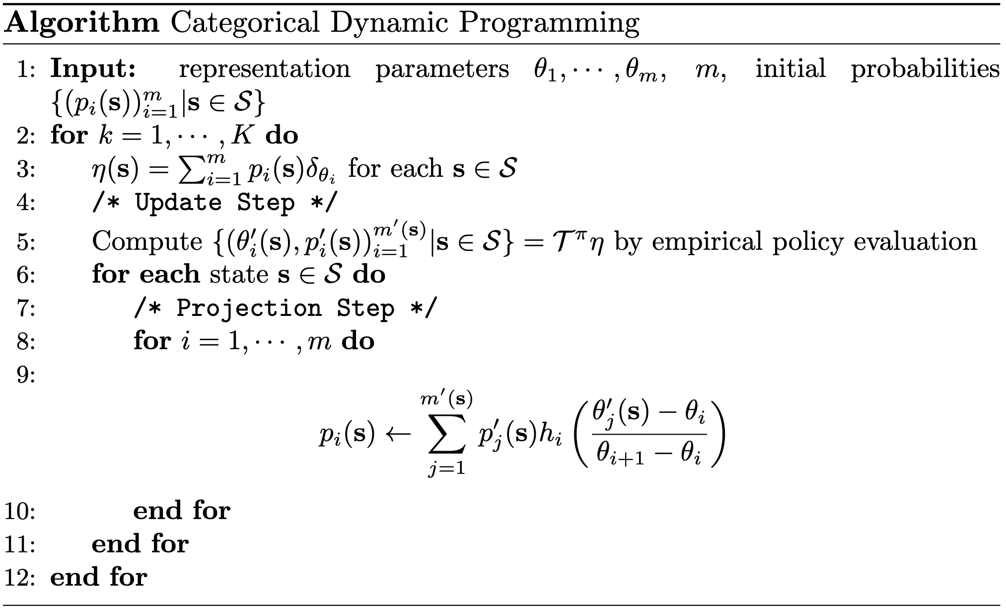
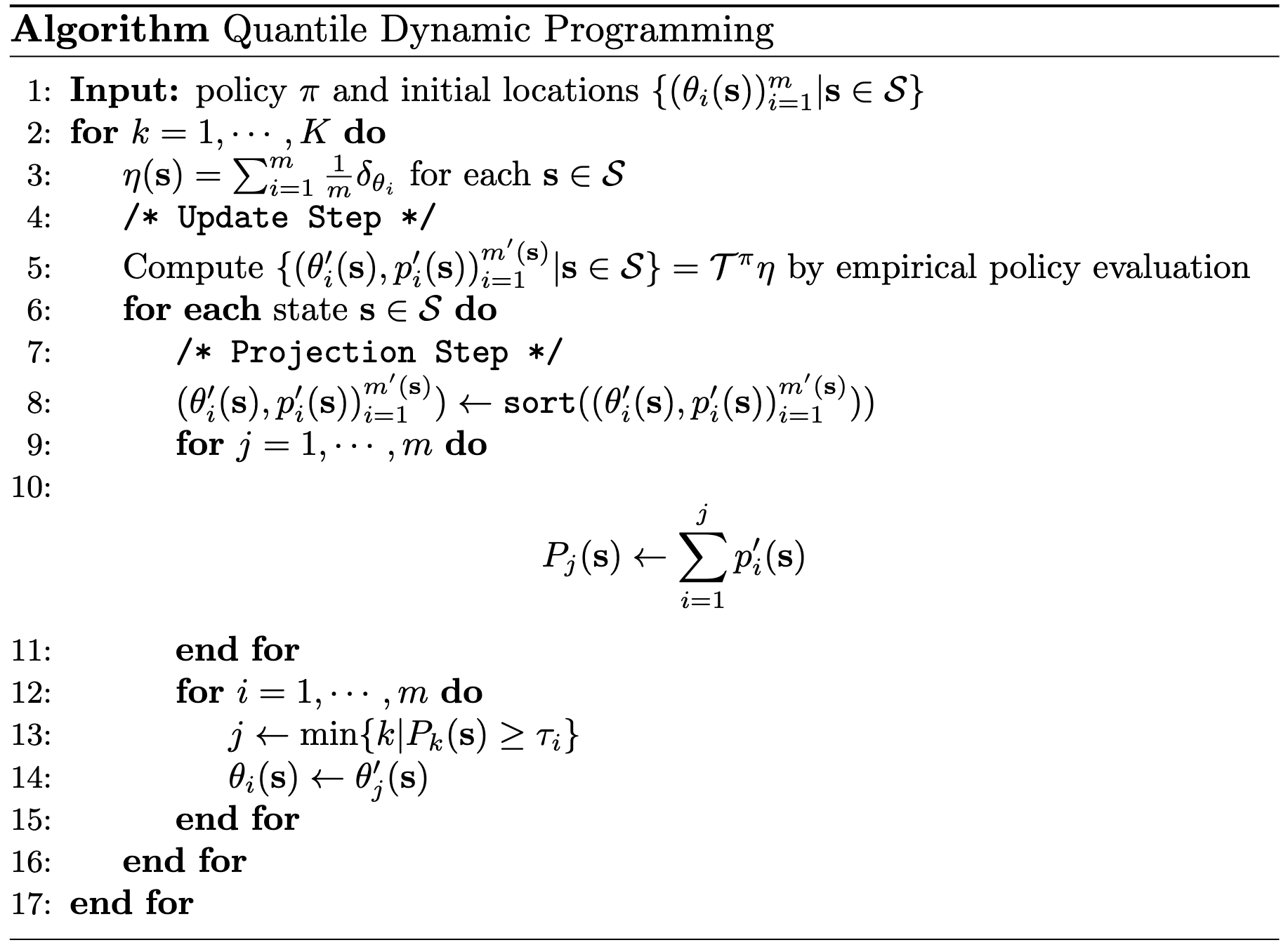
And we obtain categorical and quantile dynamic programming by applying categorical and quantile representation, respectively.
Theoritical Analysis
Although the choice of representation and projection step, arbitrary combinations of representation and projection may result in poorly behaved algorithms, while certain combinations of representation and projection will ensure desirable properties, such as a guarantee of convergence, hold.
Utilizing operator theory, one can characterize the behavior of distributional dynamic programming, including convergence rate, point of convergence, and the incurred approximation error. This theory enables us to assess how these quantities are influenced by different choices of representation and projection.
Convergence
Let $(M, d)$ be a metric space, and let $\mathcal{O}: M \to M$ be a function on this space. The Lipschitz constant of $\mathcal{O}$ under the metric $d$ is defined by $$ \Vert \mathcal{O} \Vert_d = \underset{\begin{gathered} \mathbf{x}, \mathbf{y} \in M \\ \mathbf{x} \neq \mathbf{y} \end{gathered}}{\sup} \; \frac{d (\mathcal{O}(\mathbf{x}), \mathcal{O}(\mathbf{y}))}{d (\mathbf{x}, \mathbf{y})} $$ We call the operator $\mathcal{O}$ is a non-expansion in the metric $d$ if $\Vert \mathcal{O} \Vert_d = 1$.
We estabilsh the useful lemma for analyzing compositions of two operators:
$\color{green}{\mathbf{Proof.}}$
By applying the definition of the Lipschitz constant twice, we have
\[d ( \mathcal{O}_1 \mathcal{O}_2 (\mathbf{x}), \mathcal{O}_1 \mathcal{O}_2 (\mathbf{y})) \leq \Vert \mathcal{O}_1 \Vert_d d ( \mathcal{O}_2 (\mathbf{x}), \mathcal{O}_2 (\mathbf{y})) \leq \Vert \mathcal{O}_1 \Vert_d \Vert \mathcal{O}_2 \Vert_d\]as required.
\[\tag*{$\blacksquare$}\]Again, using the Banach’s fixed point theorem, we can develop the following sufficient conditions that ensures the convergence of distributional dynamic programming:
Let $d$ be a $c$-homogeneous for some $c > 0$, regular probability metric that is $p$-convex for some $p \in [1, \infty)$ and let $(\mathscr{F}, d)$ be a complete metric space. Suppose that the finite domain $\mathscr{P}_d (\mathbb{R})^\mathcal{S}$ is closed under both projection $\Pi_\mathscr{F}$ and the Bellman operator $\mathcal{T}^\pi$: $$ \eta \in \mathscr{P}_d (\mathbb{R})^\mathcal{S} \implies \mathcal{T}^\pi \eta, \Pi_\mathscr{F} \eta \in \mathscr{P}_d (\mathbb{R})^\mathcal{S} $$ If $\Pi_\mathscr{F}$ is a non-expansion in $\bar{d}$, the corresponding projected Bellman operator $\Pi_\mathscr{F} \mathcal{T}^\pi$ has a unique fixed point $\hat{\eta}^\pi$ in $\mathscr{P}_d (\mathbb{R})^\mathcal{S}$: $$ \hat{\eta}^\pi = \Pi_\mathscr{F} \mathcal{T}^\pi \hat{\eta}^\pi $$ Additionally, for any $\varepsilon > 0$, if the $K$ the number of iterations such that $$ K \geq \frac{\log \varepsilon - \log \bar{d} (\eta_0, \hat{\eta}^\pi)}{c \log \gamma} $$ with $\eta_0 (\mathbf{s}) \in \mathscr{P}_d (\mathbb{R})$ for all $\mathbf{s} \in \mathcal{S}$, then the output $\eta_K$ of distributional dynamic programming satisfies $$ \bar{d} (\eta_K, \hat{\eta}^\pi) \leq \varepsilon $$
$\color{#bf1100}{\mathbf{Proof.}}$
Note that the conditions of $d$ are sufficient for contractability of $\mathcal{T}^\pi$ with respect to $\bar{d}$. Specifically, $\mathcal{T}^\pi$ is $\gamma^c$-contractive mapping on \(\mathscr{P}_d (\mathbb{R})^\mathcal{S}\) with respect to $\bar{d}$. In addition, since it’s trivial that \(\Pi_\mathscr{F}\) is non-expansion for any metrics $d$, the composition \(\Pi_\mathscr{F} \mathcal{T}^\pi\) is also $\gamma^c$-contractive mapping on \(\mathscr{P}_d (\mathbb{R})^\mathcal{S}\) with respect to $\bar{d}$.
By Banach’s fixed point theorem, there is a unique fixed point $\hat{\eta}^\pi$ for $\Pi_\mathscr{F} \mathcal{T}^\pi$ in $\mathscr{P}_d (\mathbb{R})^\mathcal{S}$.
Now, note that
\[\bar{d}(\eta_K, \hat{\eta}^\pi) = \bar{d}(\Pi_\mathscr{F} \mathcal{T}^\pi \eta_{K-1}, \Pi_\mathscr{F} \mathcal{T}^\pi \hat{\eta}^\pi) \leq \gamma^c \bar{d} (\eta_{K-1}, \hat{\eta}^\pi)\]By induction,
\[\bar{d}(\eta_K, \hat{\eta}^\pi) \leq \gamma^{cK} \bar{d} (\eta_0, \hat{\eta}^\pi)\]Setting the RHS to less than $\varepsilon$ and rearranging yields the result.
\[\tag*{$\blacksquare$}\]Note that the above conditions are not necessary; we can demonstrate that categorical and quantile dynamic programming is guaranteed to converge due to the contractivity of the projected distributional Bellman operator $\Pi_\mathscr{F} \mathcal{T}^\pi$.
In the case of categorical dynamic programming, we can show that the projection $\Pi_{\mathscr{F}}$ with respect to $\ell_2$ distance is non-expansion in some conditions, and the $m$-categorical representation $\mathscr{F}_{C,m}$ satisfies such conditions for all $m\in \mathbb{N}^+$:
Consider a representation $\mathscr{F} \subseteq \mathscr{P}_{\ell_2} (\mathbb{R})$. If $\mathscr{F}$ is complete with respect to $\ell_2$ and convex, then the $\ell_2$-projection $\Pi_{\mathscr{F}, \ell_2}: \mathscr{P}_{\ell_2} (\mathbb{R}) \to \mathscr{F}$ is a non-expansion in that metric: $$ \Vert \Pi_{\mathscr{F}, \ell_2} \Vert_{\ell_2} = 1 $$ Furthermore, the result extends to return functions and the supremum extension of $\ell_2$: $$ \Vert \Pi_{\mathscr{F}, \ell_2} \Vert_{\bar{\ell}_2} = 1 $$
$\color{green}{\mathbf{Proof.}}$
We will prove much general statement: finite-dimensional Euclidean projections onto closed convex sets are non-expansions. For any $\nu \in \mathscr{P}_{\ell_2} (\mathbb{R})$ and $\nu^\prime \in \mathscr{F}$, we have
\[\int_{\mathbb{R}} (F_\nu (z) - F_{\Pi \nu} (z)) (F_{\nu^\prime} (z) - F_{\Pi \nu} (z)) \mathrm{d}z \leq 0\]since if note, we have $(1 - \varepsilon) \Pi \nu + \varepsilon \nu^\prime \in \mathscr{F}$ for all $\varepsilon \in (0, 1)$ by convexity, and
\[\begin{aligned} & \ell_2^2 (\nu, (1-\varepsilon) \Pi \nu + \varepsilon \nu^\prime) \\ = & \int_{\mathbb{R}}(F_\nu (z) - (1-\varepsilon) F_{\Pi \nu}(z) - \varepsilon F_{\nu^\prime}(z))^2 \mathrm{~d} z \\ = & \ell_2^2(\nu, \Pi \nu) - 2 \varepsilon \int_{\mathbb{R}} (F_\nu (z) - F_{\Pi \nu} (z) ) (F_{\nu^\prime}(z)-F_{\Pi \nu}(z) ) \mathrm{d} z+ O(\varepsilon^2) \end{aligned}\]The last line must be at least as great as $\ell_2^2 (\nu, \Pi \nu)$ for all $\varepsilon \in (0, 1)$, by definition of $\Pi$. Therefore, it must be the case that the above inequality holds since if not, we could select $\varepsilon > 0$ sufficiently small to make $\ell_2^2 (\nu, (1 − \varepsilon) \Pi \nu + \varepsilon \nu^\prime)$ smaller than $\ell_2^2 (\nu, \Pi \nu)$.
Take $\nu_1, \nu_2 \in \mathscr{P}_{\ell_2} (\mathbb{R})$. By the inequality:
\[\begin{gathered} \int_{\mathbb{R}} (F_{\nu_1} (z) - F_{\Pi \nu_1} (z)) (F_{\Pi \nu_2} (z) - F_{\Pi \nu_1} (z)) \mathrm{d}z \leq 0 \\ \int_{\mathbb{R}} (F_{\nu_2} (z) - F_{\Pi \nu_2} (z)) (F_{\Pi \nu_1} (z) - F_{\Pi \nu_2} (z)) \mathrm{d}z \leq 0 \end{gathered}\]By adding two inequalities:
\[\begin{aligned} & \int_{\mathbb{R}} (F_{\nu_1}(z) - F_{\nu_2}(z) + F_{\Pi \nu_1}(z) - F_{\Pi \nu_2}(z)) (F_{\Pi \nu_1}(z) - F_{\Pi \nu_2}(z)) \mathrm{d} z \leq 0 \\ \Longrightarrow & \; \ell_2^2 (\Pi \nu_1, \Pi \nu_2) + \int_{\mathbb{R}} (F_{\nu_1}(z) - F_{\nu_2}(z)) (F_{\Pi \nu_1}(z) - F_{\Pi \nu_2}(z)) \mathrm{d} z \leq 0 \\ \Longrightarrow & \; \ell_2^2 (\Pi \nu_1, \Pi \nu_2) \leq \int_{\mathbb{R}} (F_{\nu_2}(z) - F_{\nu_1}(z)) (F_{\Pi \nu_1}(z) - F_{\Pi \nu_2}(z)) \mathrm{d} z. \end{aligned}\]By Cauchy-Schwartz inequality to the RHS:
\[\ell_2^2 (\Pi \nu_1, \Pi \nu_2) \leq \ell_2 (\Pi \nu_1, \Pi \nu_2) \ell_2 (\nu_1, \nu_2),\]from which the result follows by rearranging terms.
\[\tag*{$\blacksquare$}\]The $m$-categorical representation $\mathscr{F}_{C,m}$ is convex and complete with respect to the $\ell_2$ metric, for all $m \in \mathbb{N}^+$.
$\color{green}{\mathbf{Proof.}}$
Convexity
Let $f_1, f_2 \in \mathscr{F}_{C, m}$. Then, we can write $f_1$ and $f_2$ as follows:
\[\begin{aligned} f_1 & = \sum_{i=1}^m p_i \delta_{\theta_i} \text{ where } p_i \geq 0, \sum_{i=1}^m p_i = 1 \\ f_1 & = \sum_{i=1}^m q_i \delta_{\theta_i} \text{ where } q_i \geq 0, \sum_{i=1}^m q_i = 1 \\ \end{aligned}\]Let any $t \in [0, 1]$ be given. Then,
\[f = (1-t)f_1 + t f_2 = \sum_{i=1}^m ((1-t) p_i + t q_i) \delta_{\theta_i}\]If we denote by $r_i$ $(1-t) p_i + t q_i$, it is obvious that $f \in \mathscr{F}_{C, m}$.
Completeness
Let any Cauchy sequence \(\{ f_n \}\) of $(\mathscr{F}_{C, m}, \ell_2)$ be given. Let $\mathbf{p}^n \in \mathbb{R}^m$ be a vector of probabilities of $f_n$:
\[\mathbf{p}^n = (p_1^n, \cdots, p_m^n) \text{ where } f_n = \sum_{i=1}^m p_i^n \delta_{\theta_i}\]Then for any $\varepsilon > 0$, there exists $N \in \mathbb{N}$ such that for all $m, n > N$:
\[\ell_2^2 (f_k, f_l) = \sum_{i=1}^m (p_i^k - p_i^l)^2 = \Vert \mathbf{p}^k - \mathbf{p}^l \Vert_2^2 < \varepsilon^2\]Since \(\{ \mathbf{p}^n \}\) is Cauchy sequence on $(\mathbb{R}^m, \Vert \cdot \Vert_2)$ and $(\mathbb{R}^m, \Vert \cdot \Vert_2)$ is complete, there exists a limit
\[\mathbf{p} = \lim_{n \to \infty} \mathbf{p}^n = (p_1, \cdots, p_m) \text{ where } \sum_{i=1}^m p_i = \sum_{i=1}^m \lim_{n \to \infty} p_i^n = \lim_{n \to \infty} \sum_{i=1}^m p_i^n = 1\]Writing $f = \sum_{i=1}^m p_i \delta_{\theta_i}$, it is obvious that $\lim_{n \to \infty} f_n = f$ with respect to $\ell_2$ metric and $f_n \in \mathscr{F}_{C, m}$ as required.
\[\tag*{$\blacksquare$}\]In case of quantile representation, we can show that the $W_1$-projected distributional Bellman operator $\Pi_Q \mathcal{T}^\pi$ is $\gamma$-contraction with respect to \(\overline{W}_\infty\) by showing that $W_1$-projection $\Pi_Q$ is non-expansion in $W_\infty$:
Assume that the finite domain $\mathscr{P}_{W_\infty} (\mathbb{R})^\mathcal{S}$ is closed under both the projection $\Pi_Q$ and the Bellman operator $\mathcal{T}^\pi$: $$ \eta \in \mathscr{P}_d (\mathbb{R})^\mathcal{S} \implies \mathcal{T}^\pi \eta, \Pi_Q \eta \in \mathscr{P}_d (\mathbb{R})^\mathcal{S} $$ Then, the $W_1$-projection $\Pi_Q$ is non-expansion in $W_\infty$: $$ \Vert \Pi_Q \Vert_{W_\infty} = 1 $$ and the projected distributional Bellman operator $\Pi_Q \mathcal{T}^\pi: \mathscr{P}_{W_\infty} (\mathbb{R})^\mathcal{S} \to \mathscr{P}_{W_\infty} (\mathbb{R})^\mathcal{S}$ is $\gamma$-contraction mapping in $\overline{W}_\infty$: $$ \Vert \Pi_Q \mathcal{T}^\pi \Vert_{\overline{W}_\infty} \leq \gamma $$
$\color{green}{\mathbf{Proof.}}$
Since $\mathcal{T}^\pi$ is a $\gamma$-contraction in \(\overline{W}_\infty\), it suffices to show that \(\Pi_Q: \mathscr{P}_{W_\infty} (\mathbb{R}) \to \mathscr{P}_{W_\infty} (\mathbb{R})\) is a non-expansion in $W_\infty$; the result then follows from the inequality for Lipschitz constant of composition of operators.
For any \(\nu_1, \nu_2 \in \mathscr{P}_{W_\infty} (\mathbb{R})\), we have
\[W_\infty (\nu_1, \nu_2) = \underset{\tau \in (0, 1)}{\sup} \vert F_{\nu_1}^{-1} (\tau) - F_{\nu_2}^{-1} (\tau) \vert\]Note that
\[\begin{aligned} \Pi_Q \nu_1 & = \frac{1}{m} \sum_{i=1}^m \delta_{F_{\nu_1}^{-1} (\tau_i)} \\ \Pi_Q \nu_2 & = \frac{1}{m} \sum_{i=1}^m \delta_{F_{\nu_2}^{-1} (\tau_i)} \end{aligned}\]where $\tau_i = \frac{2i-1}{2m}$. Then we have
\[\begin{aligned} W_\infty (\Pi_Q \nu_1, \Pi_Q \nu_2) & = \underset{i=1, \cdots, m}{\max} \vert F_{\nu_1}^{-1} (\tau_i) - F_{\nu_2}^{-1} (\tau_i) \vert \\ & \leq \underset{\tau \in (0, 1)}{\sup} \vert F_{\nu_1}^{-1} (\tau) - F_{\nu_2}^{-1} (\tau) \vert = W_\infty (\nu_1, \nu_2) \end{aligned}\]as required.
\[\tag*{$\blacksquare$}\]Approximation Error Bound
Having identified the existence of converging fixed point, we need to the measure the quality of convergence compared to the true return-distribution function $\eta^\pi$. And using a representation and projection also necessarily incurs some approximation error relative to the true return function. This section analyzes quantitative bounds on such approximation error.
Let $d$ be a $c$-homogeneous for some $c > 0$, regular probability metric that is $p$-convex for some $p \in [1, \infty)$ and let $(\mathscr{F}, d)$ be a complete metric space. Suppose that the finite domain $\mathscr{P}_d (\mathbb{R})^\mathcal{S}$ is closed under both projection $\Pi_\mathscr{F}$ and the Bellman operator $\mathcal{T}^\pi$: $$ \eta \in \mathscr{P}_d (\mathbb{R})^\mathcal{S} \implies \mathcal{T}^\pi \eta, \Pi_\mathscr{F} \eta \in \mathscr{P}_d (\mathbb{R})^\mathcal{S} $$ If $\Pi_\mathscr{F}$ is a non-expansion in $\bar{d}$, a unique fixed point $\hat{\eta}^\pi \in \mathscr{P}_d (\mathbb{R})^\mathcal{S}$ of the corresponding projected Bellman operator $\Pi_\mathscr{F} \mathcal{T}^\pi$ has the following error bound: $$ \bar{d}(\hat{\eta}^\pi, \eta^\pi) \leq \frac{\bar{d} (\Pi_\mathscr{F} \eta^\pi, \eta^\pi)}{1 - \gamma^c} $$
$\color{#bf1100}{\mathbf{Proof.}}$
From the proposition, we immediately deduce a result regarding the fixed point $\hat{\eta}^\pi$ of the categorical dynamic programming of the projected operator $\Pi_C \mathcal{T}^\pi$. Although both the memory and time complexity of the representation grow with $m$, the result indicates that increasing $m$ simultaneously diminishes the approximation error arising from dynamic programming.
The fixed point $\hat{\eta}^\pi$ of the categorical-projected Bellman operator $\Pi_C \mathcal{T}^\pi: \mathscr{P}_{\ell_2} (\mathbb{R}) \to \mathscr{P}_{\ell_2} (\mathbb{R})$ satisfies $$ \bar{\ell}_2 (\hat{\eta}^\pi, \eta^\pi) \leq \frac{\bar{\ell}_2 (\Pi_C \eta^\pi, \eta^\pi)}{1 - \gamma^{1/2}} $$ If the return distributions $$\{\eta^\pi (\mathbf{s}) \vert \mathbf{s} \in \mathcal{S}\}$$ are supported on $[ \theta_1, \theta_m ]$ where the support $\theta_1, \cdots, \theta_m$ is evenly spaced, i.e. $\varsigma_i = \frac{\theta_m - \theta_1}{m-1}$ for all $i \in [1, m]$, we further obtain that for each $\mathbf{s} \in \mathcal{S}$: $$ \underset{\nu \in \mathscr{F}_{C, m}}{\min} \ell_2^2 (\nu, \eta^\pi (\mathbf{s})) \leq \varsigma_m \sum_{i=1}^m \left( F_{\eta^\pi (\mathbf{s})} (\theta_1 + i \varsigma_m) - F_{\eta^\pi (\mathbf{s})} (\theta_1 + (i - 1) \varsigma_m) \right)^2 \leq \varsigma_m $$ and hence $$ \bar{\ell}_2 (\hat{\eta}^\pi, \eta^\pi) \leq \frac{1}{1 - \gamma^{1/2}} \frac{\theta_m - \theta_1}{m-1} $$
To develop a guarantee of the approximation error incurred by the fixed point $\hat{\eta}^\pi$ of the projected distributional Bellman operator $\Pi_Q \mathcal{T}^\pi$ and the $m$-quantile representation, we can derive the error bound with respect to $W_1$:
Suppose that for each $(\mathbf{s}, \mathbf{a}) \in \mathcal{S} \times \mathcal{A}$, the reward distribution $\mathbb{P}_\mathcal{R} (\cdot \vert \mathbf{s}, \mathbf{a})$ is supported on the interval $[R_\min, R_\max]$. Then, the $m$-quantile fixed point $\hat{\eta}^\pi$ satisfies $$ \overline{W}_1 (\hat{\eta}^\pi, \eta^\pi) \leq \frac{3(V_\max - V_\min)}{2m (1-\gamma)}. $$ where $V_\min = R_\min / (1-\gamma)$ and $V_\max = R_\max / (1-\gamma)$. Furthermore, consider an initial return-distribution function $\eta_0$ with distributions with support bounded in $[V_\min, V_\max]$ an the iterates $$ \eta_{k+1} = \Pi_Q \mathcal{T}^\pi \eta_k $$ produced by quantile dynamic programming. Then, we have for all $k \geq 0$: $$ \overline{W}_1 (\eta_k, \eta^\pi) \leq \gamma^k (V_\max - V_\min) + \frac{3(V_\max - V_\min)}{2m (1-\gamma)}. $$
$\color{#bf1100}{\mathbf{Proof.}}$
Denote by \(\mathscr{P}_B (\mathbb{R})\) the space of probability distributions bounded on $[V_\min, V_\max]$. For any $\nu \in \mathscr{P}_B(\mathbb{R})$ and the quantile projection $\Pi_Q$, observe that
\[W_1 (\Pi_Q \nu, \nu) \leq \frac{V_\max - V_\min}{2m}.\]Using the triangle inequality twice, for any $\nu, \nu^\prime \in \mathscr{P}_B (\mathbb{R})$:
\[\begin{aligned} W_1 (\Pi_Q \nu, \Pi_Q \nu^\prime) & \leq W_1 (\Pi_Q \nu, \nu) + W_1 (\nu, \Pi_Q \nu^\prime) \\ & \leq \frac{V_\max - V_\min}{2m} + W_1 (\nu, \Pi_Q \nu^\prime) \\ & \leq \frac{V_\max - V_\min}{2m} + W_1 (\nu, \nu^\prime) + W_1(\nu^\prime + \Pi_Q \nu^\prime) \\ & \leq \frac{V_\max - V_\min}{m} + W_1 (\nu, \nu^\prime) \end{aligned}\]Again, using the triangle inequality with the return-distribution functions $\hat{\eta}^\pi$, $\Pi_Q \eta^\pi$, and $\eta^\pi$ and the fact that $\Pi_Q \mathcal{T}^\pi \hat{\eta}^\pi = \hat{\eta}^\pi$ and $\mathcal{T}^\pi \eta^\pi = \eta^\pi$, we demonstrate that if $\eta^\pi \in \mathscr{P}_B (\mathbb{R})^\mathcal{S}$, then we have
\[\begin{aligned} \overline{W}_1 (\hat{\eta}^\pi, \eta^\pi) & \leq \overline{W}_1 (\hat{\eta}^\pi, \Pi_Q \eta^\pi) + \overline{W}_1 (\Pi_Q \eta^\pi, \eta^\pi) \\ & \leq \overline{W}_1 (\hat{\eta}^\pi, \Pi_Q \eta^\pi) + \frac{V_\max - V_\min}{2m} \\ & = \overline{W}_1 (\Pi_Q \mathcal{T}^\pi \hat{\eta}^\pi, \Pi_Q \mathcal{T}^\pi \eta^\pi) + \frac{V_\max - V_\min}{2m} \\ & \leq \frac{3(V_\max - V_\min)}{2m} + \overline{W}_1 (\mathcal{T}^\pi \hat{\eta}^\pi, \mathcal{T}^\pi \eta^\pi) \\ & \leq \frac{3(V_\max - V_\min)}{2m} + \gamma \overline{W}_1 (\hat{\eta}^\pi, \eta^\pi) \end{aligned}\]therefore
\[\overline{W}_1 (\hat{\eta}^\pi, \eta^\pi) \leq \frac{3(V_\max - V_\min)}{2m(1-\gamma)}.\]Observing that $W_1 (\nu, \nu^\prime) \leq W_\infty (\nu, \nu^\prime)$ for any $\nu, \nu^\prime \in \mathscr{P}_B(\mathbb{R})$, from the triangle inequality
\[\overline{W}_1 (\eta_k, \eta^\pi) \leq \overline{W}_1 (\eta_k, \hat{\eta}^\pi) + \overline{W}_1 (\hat{\eta}^\pi, \eta^\pi)\]we deduce that
\[\overline{W}_1 (\eta_k, \eta^\pi) \leq \gamma^k (V_\max - V_\min) + \frac{3(V_\max - V_\min)}{2m(1-\gamma)}\]from the induction.
\[\tag*{$\blacksquare$}\]References
[1] Marc G. Bellemare and Will Dabney and Mark Rowland, “Distributional Reinforcement Learning”, MIT Press 2023
[2] Rowland et al. “An Analysis of Categorical Distributional Reinforcement Learning”, PMLR 2018
[3] Bellemare et al. “A Distributional Perspective on Reinforcement Learning”, ICML 2017
[4] Rowland et al. “Statistics and Samples in Distributional Reinforcement Learning”, PMLR 2019
Leave a comment