[RL] Deep Distributional RL

Beginning around 2013, DeepMind demonstrated impressive learning results using deep RL, called Deep Q-Network (DQN), to play Atari video games. And several milestones such as AlphaGo positioned deep reinforcement learning as a promising solution for various RL tasks.

Building on this trend, much of the recent research in distributional reinforcement learning is also rooted in deep reinforcement learning. This post discusses some notable works in deep distributional RL, which originated from DQN.

$\mathbf{Fig\ 1.}$ Deep Distributional DQNs (Dabney et al., ICML 2018)

Preliminary: DQN

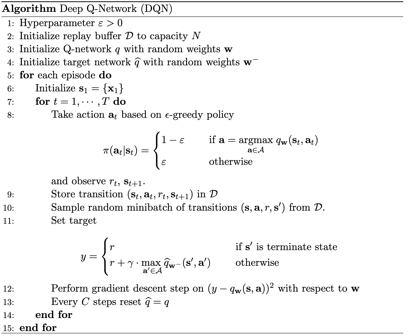
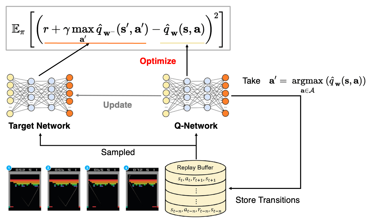
Recall that the computation of Deep Q-Network (DQN) consists of 4 components:

• (a) Preprocess: convert observations (Atari 2600 images) into input vectors
• (b) Prediction: predict the expected return from the agent’s current state
• (c) Action: behave on the basis of the predictions
• (d) Learning: improve the agent’s predictions from its experience

$\mathbf{Fig\ 2.}$ The pseudocode for Deep Q-Network

Specifically:

1. Prediction
   Using Q-network $Q_\mathbf{w}$, DQN predicts the expected return of the possible actions $\mathbf{a}_t \in \mathcal{A}$ given state $\mathbf{s}_t$ by $Q_\mathbf{w} (\mathbf{s}_t, \mathbf{a}_t)$.
2. Action
   The DQN agent follows an $\varepsilon$-greedy policy: $$ \pi (\mathbf{a}_t \vert \mathbf{s}_t) = \begin{cases} 1 - \varepsilon & \quad \text{ if } \mathbf{a}_t = \underset{\mathbf{a} \in \mathcal{A}}{\arg \max} \; Q_\mathbf{w} (\mathbf{s}_t, \mathbf{a}) \\ \varepsilon & \quad \text{ otherwise } \end{cases} $$ And the agent observes $r_t$, $\mathbf{s}_{t+1}$ and stores transition $(\mathbf{s}_t, \mathbf{a}_t, r_t, \mathbf{s}_{t+1})$ in replay buffer $\mathcal{D}$.
3. Learning
   To ensure the independency in the gradient descent algorithm, sample random transition $(\mathbf{s}, \mathbf{a}, r, \mathbf{s}^\prime) \sim \mathcal{D}$ first. Then, using target network $Q_{\tilde{\mathbf{w}}}$, the target value for Q-network is set to: $$ y = \begin{cases} r & \quad \text{ if } \mathbf{s}^\prime \text{ is terminal state } \\ r + \gamma \underset{\mathbf{a}^\prime \in \mathcal{A}}{\max} \; Q_{\tilde{\mathbf{w}}}(\mathbf{s}^\prime, \mathbf{a}^\prime) & \quad \text{ otherwise } \end{cases} $$ Then, the parameters of networks are updated as follows: $$ \begin{aligned} \mathbf{w} & \leftarrow \mathbf{w} + \eta_{\mathbf{w}} \nabla_\mathbf{w} (y - Q_\mathbf{w} (\mathbf{s}, \mathbf{a}))^2 \\ \tilde{\mathbf{w}} & \leftarrow \mathbf{w} \text{ for every } C > 1 \text{ step } \end{aligned} $$

$\mathbf{Fig\ 3.}$ Deep Q-Network Framework

Categorical DQN (C51)

The Categorical DQN (C51) algorithm is the first extension of DQN to the distributional setting, introduced in Bellemare et al., ICML 2017. It is termed C51 because it employs a $51$-categorical representation in its original implementation, but an abitrary number of categories are possible to use.

The original implementation of C51 parameterizes the support \(\{ \theta_i \}_{i=1}^m\) in two sepecific ways:

• $\theta_1 = V_\min = - \theta_m = - V_\max$, therefore the support is symmetric around $0$;
• $m$ is set to odd numbers so that the center $\theta_{\frac{m-1}{2}} = 0$;

And recall that the categorical projection $\Pi_C$ allocates probability mass $p_i$ from $\nu$ to the location $\theta_i$ in proportion to the distance to its adjacent point:

\[\Pi_c \nu = \sum_{i=1}^m p_i \delta_{\theta_i}\]

where

\[p_i = \mathbb{E}_{Z \sim \nu} \left[h_i \left( \frac{Z - \theta_i}{\varsigma_i = \theta_{i+1} - \theta_{i}} \right) \right]\]

using a set of triangle kernels $h_i: \mathbb{R} \to [0, 1]$ that converts the length to the probability:

\[\begin{aligned} h_1 (z) & = \begin{cases} 1 & \quad z \leq 0 \\ \max (0, 1 - \vert z \vert) & \quad z > 0 \end{cases} \\ h_2 (z) & = \cdots = h_{m-1} (z) = \max (0, 1 - \vert z \vert) \\ h_m (z) & = \begin{cases} \max (0, 1 - \vert z \vert) & \quad z \leq 0 \\ 1 & \quad z > 0 \end{cases} \end{aligned}\]

Instead of using $h_1$ and $h_m$, we can bound the support $\nu$ by $[\theta_1 = V_\min, \theta_m = V_\max]$.

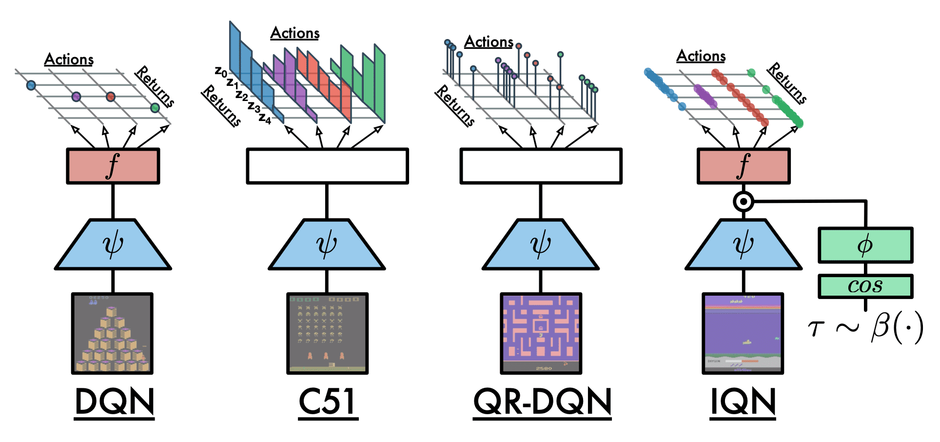
The overall C51 algorithm is illustrated below compared to the DQN:

1. Prediction
   The Q-network $Q_\mathbf{w} (\mathbf{s}, \mathbf{a})$ of C51 outputs a collection of softmax parameters $\{ \varphi_i (\mathbf{s}, \mathbf{a}) \}_{i=1}^m$ to define the state-action categorical return distribution: $$ \eta_\mathbf{w} (\mathbf{s}, \mathbf{a}) = \sum_{i=1}^m p_i (\mathbf{s}, \mathbf{a}; \mathbf{w}) \delta_{\theta_i} $$ where $p_i (\mathbf{s}, \mathbf{a} ; \mathbf{w})$ is given by $$ p_i (\mathbf{s}, \mathbf{a}; \mathbf{w}) = \texttt{softmax} (\varphi_i (\mathbf{s}, \mathbf{a})) = \frac{\exp (\varphi_i (\mathbf{s}, \mathbf{a}))}{\sum_{j=1}^m \exp (\varphi_j (\mathbf{s}, \mathbf{a}))} $$ That is: $$ Q_\mathbf{w} (\mathbf{s}, \mathbf{a}) = \mathbb{E}_{Z \sim \eta_\mathbf{w} (\mathbf{s}, \mathbf{a})} [Z] = \sum_{i=1}^m p_i (\mathbf{s}, \mathbf{a} ; \mathbf{w}) \theta_i $$
2. Action
   The C51 agent also follows an $\varepsilon$-greedy policy: $$ \pi (\mathbf{a}_t \vert \mathbf{s}_t) = \begin{cases} 1 - \varepsilon & \quad \text{ if } \mathbf{a}_t = \underset{\mathbf{a} \in \mathcal{A}}{\arg \max} \; Q_\mathbf{w} (\mathbf{s}_t, \mathbf{a}) \\ \varepsilon & \quad \text{ otherwise } \end{cases} $$ And the agent observes $r_t$, $\mathbf{s}_{t+1}$ and stores transition $(\mathbf{s}_t, \mathbf{a}_t, r_t, \mathbf{s}_{t+1})$ in replay buffer $\mathcal{D}$.
3. Learning
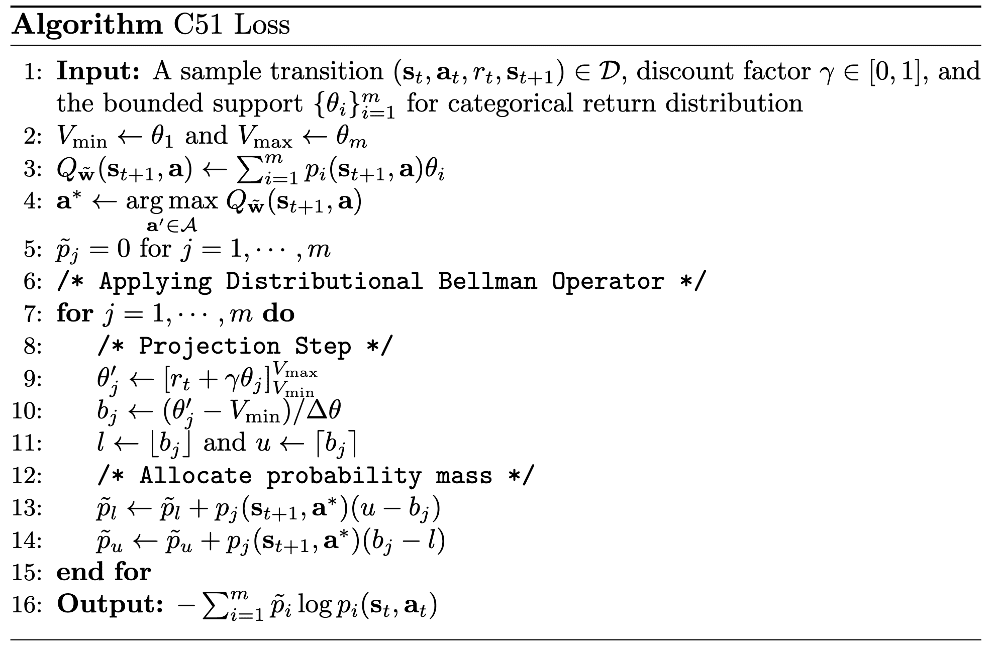
   From random transition $(\mathbf{s}, \mathbf{a}, r, \mathbf{s}^\prime) \sim \mathcal{D}$, the target value for Q-network is set by target network $Q_{\tilde{\mathbf{w}}}$: $$ \bar{\eta} (\mathbf{s}, \mathbf{a}) = \Pi_C \left[ (b_{r, \gamma})_* (\eta_{\tilde{\mathbf{w}}}) (\mathbf{s}^\prime, \mathbf{a}_{\tilde{\mathbf{w}}} (\mathbf{s}^\prime)) \right] = \sum_{j=1}^m \tilde{p}_j \delta_{\theta_j} $$ where $$ \mathbf{a}_{\tilde{\mathbf{w}}} (\mathbf{s}^\prime) = \underset{\mathbf{a}^\prime \in \mathcal{A}}{\arg \max} \; Q_{\tilde{\mathbf{w}}} (\mathbf{s}^\prime, \mathbf{a}^\prime) $$ and for $\texttt{bound}$ operation $[ \cdot ]_a^b: \mathbb{R} \to [a, b]$: $$ \tilde{p}_j = \sum_{i = 1}^m \left[ 1 - \frac{ \lvert [ r + \gamma \theta_i ]_{V_\min}^{V_\max} - \theta_j \rvert }{\Delta \theta = \theta_{j + 1} - \theta_j} \right]_0^1 \times p_i (\mathbf{s}^\prime, \mathbf{a}_{\tilde{\mathbf{w}}} (\mathbf{s}^\prime); \tilde{\mathbf{w}}) $$ Then, the cross-entropy loss is leveraged to optimize the Q-network which is equivalent to the KL divergence between two return distributions: $$ \begin{aligned} \mathcal{L}(\mathbf{w}) & = - \sum_{j=1}^m \tilde{p}_j \log p_j (\mathbf{s}, \mathbf{a} ; \mathbf{w}) \\ & = \mathrm{KL} ( \Pi_C \left[ (b_{r, \gamma})_* (\eta_{\tilde{\mathbf{w}}}) (\mathbf{s}^\prime, \mathbf{a}_{\tilde{\mathbf{w}}} (\mathbf{s}^\prime)) \right] \Vert \eta_{\mathbf{w}} (\mathbf{s}, \mathbf{a}) ) \end{aligned} $$

The following pseudocode computes the C51 loss by processing the projection in $\mathcal{O}(m)$:

$\mathbf{Fig\ 4.}$ The pseudocode for computing C51 loss. (Bellemare et al., 2017)

Using more atoms $\theta$ consistently enhances performance, and as the name C51 implies, the $51$-atom version demonstrated the best results among other variants. Furthermore, the difference in performance between C51 and DQN is particularly striking and achieves the state-of-the-art performance.

$\mathbf{Fig\ 5.}$ Varying number of atoms in the discrete distribution. Scores are moving averages over 5 million frames. (Bellemare et al., 2017)

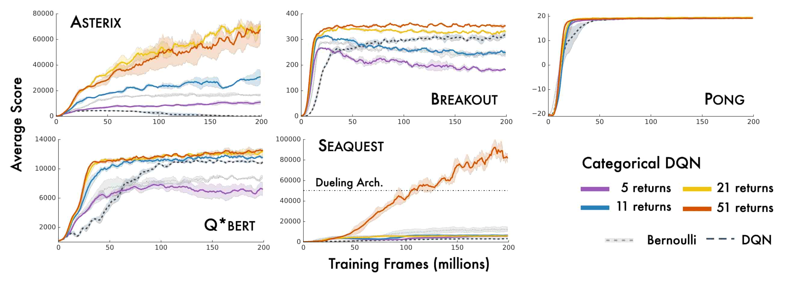
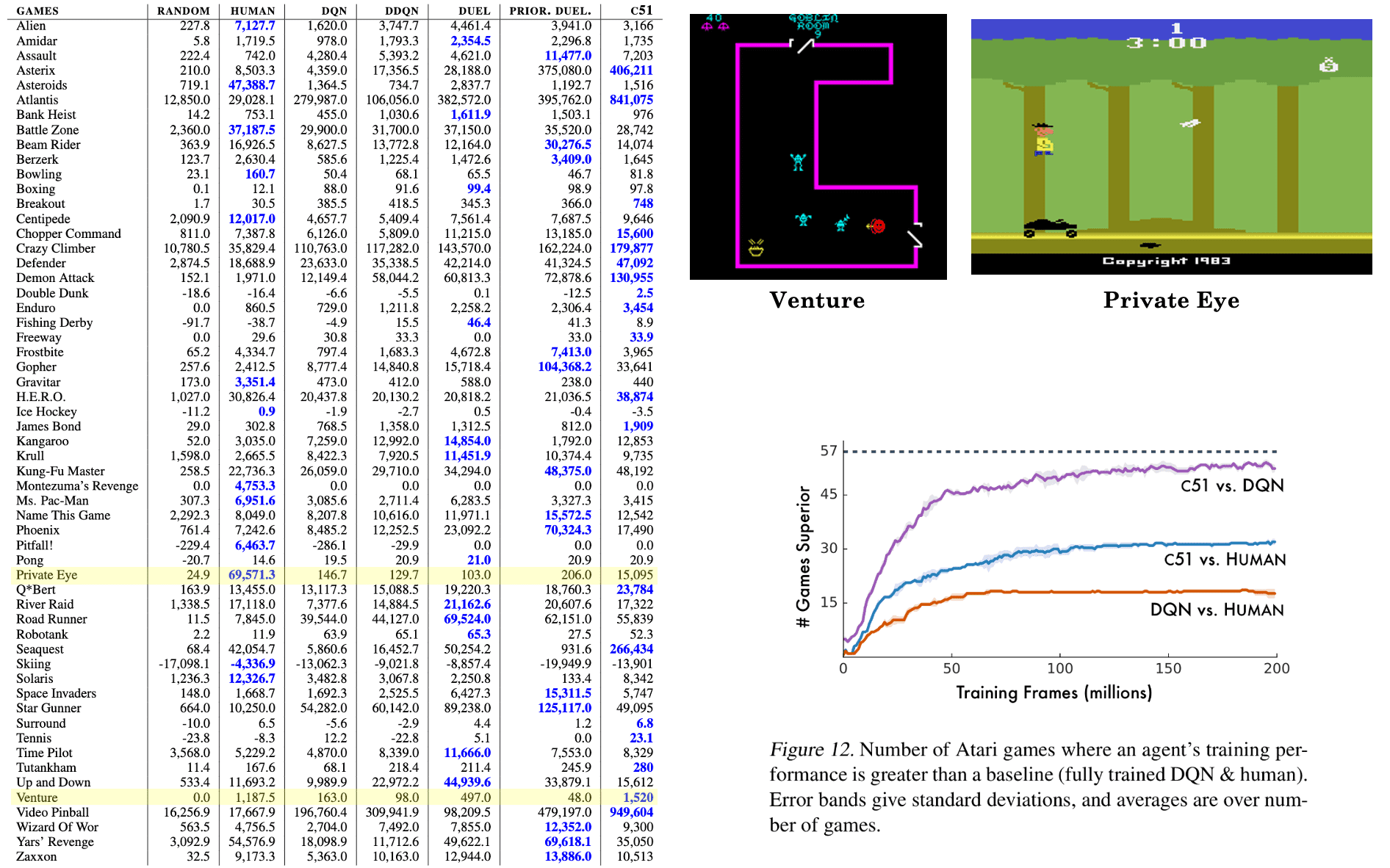
One notable fact is the C51’s good performance on sparse reward games such as VENTURE and PRIVATE EYE. This suggests that value distributions are better able to propagate rarely occurring events. Consequently, the number of games in which C51’s training performance surpasses that of fully-trained DQN and human players is significant.

$\mathbf{Fig\ 6.}$ Comparisons of C51 (Bellemare et al., 2017)

Quantile Regression DQN (QR-DQN)

Although the convergence of the distributional optimality operator is guaranteed regarding the supremum extension of Wasserstein distance $\bar{W}_p$ under some conditions, the C51 minimizes KL divergence instead due to practical reasons.

Moreover, the categorical parameterization requires its fixed locations that restricts the support to be within pre-defined bound and the uniform resolution and also necessitates the domain knowledge about the bounds of the return distribution.

Instead of categorical distribution, Quantile Regression DQN (QR-DQN) approximates the return distribution at each state-action using quantile.

• Advantages over C51
  • The support is not restricted to prespecified bounds or a uniform resolution;
  • The quantile projection $\Pi_Q$ is more manageable than $\Pi_C$;
  • Approxmately minimizes $W_1$ metric with the optimal distribution using quantile regression;

Preliminary: Quantile Regression

Quantile regression is a method for determining the quantiles of a probability distribution incrementally and from samples. Formally, for given $\tau \in (0,1)$, it aims to estimate the $\tau$-th quantile of the distribution $\nu$, corresponding to $F_\nu^{-1} (\tau)$, with the following incremental update:

\[\theta \leftarrow \theta + \alpha (\tau - \mathbf{1}_{\{z < \theta\}})\]

where $z \sim \nu$ is sampled from $\nu$. It is equivalent to the gradient descent of the quantile regression loss:

\[\begin{aligned} \mathcal{L}_\tau (\theta) & = (\tau - \mathbf{1}_{\{z < \theta\}})(z - \theta) \\ & = \vert \mathbf{1}_{\{z < \theta\}} - \tau \vert \times \vert z - \theta \vert \end{aligned}\]

It is an asymmetric convex loss function that penalizes overestimation errors with a weight of $\tau$ and underestimation errors with a weight of $1 - \tau$.

It is obivious that the equilibrium point $\theta^*$ of the update is the true quantile $F_\nu^{-1} (\tau)$:

\[\begin{gathered} \begin{aligned} 0 & = \mathbb{E}_{Z \sim \nu} [\tau - \mathbf{1}_{\{z < \theta\}}] \\ & = \tau - \mathbb{E}_{Z \sim \nu} [\mathbf{1}_{\{z < \theta\}}] \\ & = \tau - \mathbb{P}(Z < \theta^*) \end{aligned} \\ \therefore \mathbb{P}(Z < \theta^*) = \tau \end{gathered}\]

Quantile Temporal-Difference Learning (QTD)

To find a $m$-qunatile approximation to the return-distribution fuction $\eta$:

\[\eta (\mathbf{s}) = \frac{1}{m} \sum_{i=1}^m \delta_{\theta_i (\mathbf{s})}\]

quantile regression can be applied. To perform quantile regression for all location parameters \(\{ \theta_i \}_{i=1}^m\) that estimates the quantile levels \(\{ \tau_i \}_{i=1}^m\) simultaneously, we can introduce the additional uniform random variable $J \sim \mathcal{U} (\mathcal{I})$ for indices \(\mathcal{I} = \{ 1, \cdots, m \}\). Therefore:

\[(R + \gamma \theta_J (\mathbf{S}^\prime) \vert \mathbf{S} = \mathbf{s}, \mathbf{A} \sim \pi) \sim (\mathcal{T}^\pi \eta) (\mathbf{s})\]

For given transition $(\mathbf{s}, \mathbf{a}, r, \mathbf{s}^\prime)$, the update rule can be constructed by quantile regression, using $m$ sample targets \(\{r + \gamma \theta_j (\mathbf{s}^\prime) \}_{j=1}^m\):

\[\theta_i (\mathbf{s}) \leftarrow \theta_i (\mathbf{s}) + \frac{\alpha}{m} \sum_{j=1}^m \left( \tau_i - \mathbf{1}_{\{ r + \gamma \theta_j (\mathbf{s}^\prime) < \theta_i (\mathbf{s}) \}} \right) \quad \forall i \in \{ 1, \cdots, m \}\]

which optimizes $\theta_i (\mathbf{s})$ to be

\[\theta_i^* (\mathbf{s}) = F_{\mathcal{T}^\pi \eta (\mathbf{s})}^{-1} (\tau_i)\]

This is known as quantile (regression) temporal-difference learning.

Algorithm

The overall QR-DQN algorithm is illustrated below compared to the DQN:

1. Prediction
   The Q-network $Q_\mathbf{w} (\mathbf{s}, \mathbf{a})$ of QR-DQN outputs a collection of atoms $\{ \theta_i (\mathbf{s}, \mathbf{a}; \mathbf{w}) \}_{i=1}^m$ to define the state-action quantile return distribution: $$ \eta_\mathbf{w} (\mathbf{s}, \mathbf{a}) = \sum_{i=1}^m \frac{1}{m} \delta_{\theta_i (\mathbf{s}, \mathbf{a}; \mathbf{w})} $$ where its induce Q-value function is simply: $$ Q_\mathbf{w} (\mathbf{s}, \mathbf{a}) = \mathbb{E}_{Z \sim \eta_\mathbf{w} (\mathbf{s}, \mathbf{a})} [Z] = \sum_{i=1}^m \frac{1}{m} \theta_i (\mathbf{s}, \mathbf{a}; \mathbf{w}) $$
2. Action
   The QR-DQN agent also follows an $\varepsilon$-greedy policy: $$ \pi (\mathbf{a}_t \vert \mathbf{s}_t) = \begin{cases} 1 - \varepsilon & \quad \text{ if } \mathbf{a}_t = \underset{\mathbf{a} \in \mathcal{A}}{\arg \max} \; Q_\mathbf{w} (\mathbf{s}_t, \mathbf{a}) \\ \varepsilon & \quad \text{ otherwise } \end{cases} $$ And the agent observes $r_t$, $\mathbf{s}_{t+1}$ and stores transition $(\mathbf{s}_t, \mathbf{a}_t, r_t, \mathbf{s}_{t+1})$ in replay buffer $\mathcal{D}$.
3. Learning
   Since the quantile regression loss is not smooth as $z - \theta \to 0$, QR-DQN employs a smoothed version of quantile regression loss called quantile Huber loss $\mathcal{L} (\mathbf{w})$ for sampled transition $(\mathbf{s}, \mathbf{a}, r, \mathbf{s}^\prime) \sim \mathcal{D}$: $$ \begin{gathered} \mathcal{L} (\mathbf{w}) = \frac{1}{m} \sum_{i = 1}^m \sum_{j = 1}^m \rho_{\tau_i}^\kappa ( r + \gamma \theta_j (\mathbf{s}^\prime, \mathbf{a}_{\tilde{\mathbf{w}}} (\mathbf{s}^\prime); \tilde{\mathbf{w}}) - \theta_i (\mathbf{s}, \mathbf{a} ; \mathbf{w})) \\ \text{ where } \mathbf{a}_{\tilde{\mathbf{w}}} (\mathbf{s}^\prime) = \underset{\mathbf{a}^\prime \in \mathcal{A}}{\arg \max} \; Q_\tilde{\mathbf{w}} (\mathbf{s}^\prime, \mathbf{a}^\prime) \text{ and } \rho_\tau^\kappa (u) = \vert \tau - \mathbf{1}_{u < 0} \vert \mathcal{H}_\kappa (u) \end{gathered} $$ with the quantile levels $$ \tau_i = \frac{2i - 1}{2m} $$ and Huber loss $\mathcal{H}_\kappa$: $$ \mathcal{H}_\kappa (u) = \begin{cases} \frac{1}{2} u^2 & \quad \text{ if } u \in [-\kappa, \kappa] \\ \kappa (\vert u \vert - \frac{1}{2} \kappa) & \quad \text{ otherwise } \end{cases} $$ The Huber loss corresponds to the squared loss for small errors within $\kappa$ but behaves like the quantile loss for larger errors. This effectively limits the magnitude of updates to the weight vector, thereby reducing instability in the learning process.
   
   

   

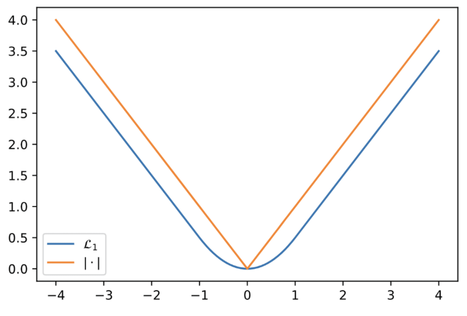
   $\mathbf{Fig\ 7.}$ Visualization of Huber loss with $\kappa = 1$ v.s. $y = \vert x \vert$
   
   Recall that $W_1$-quantile projection of $\nu$ is given by: $$ \Pi_{Q} \nu = \frac{1}{m} \sum_{i=1}^m \delta_{\theta_i} \text{ where } \theta_i = F_\nu^{-1} \left( \frac{2i-1}{2m} \right) $$ Therefore, QR-DQN is minimizing the Wasserstein loss between the optimal return distribution and the quantile approximation of Q-network.

The overall algorithm for computing the QR-DQN loss is given by the following pseudocode:

$\mathbf{Fig\ 8.}$ The pseudocode for computing QR-DQN loss.

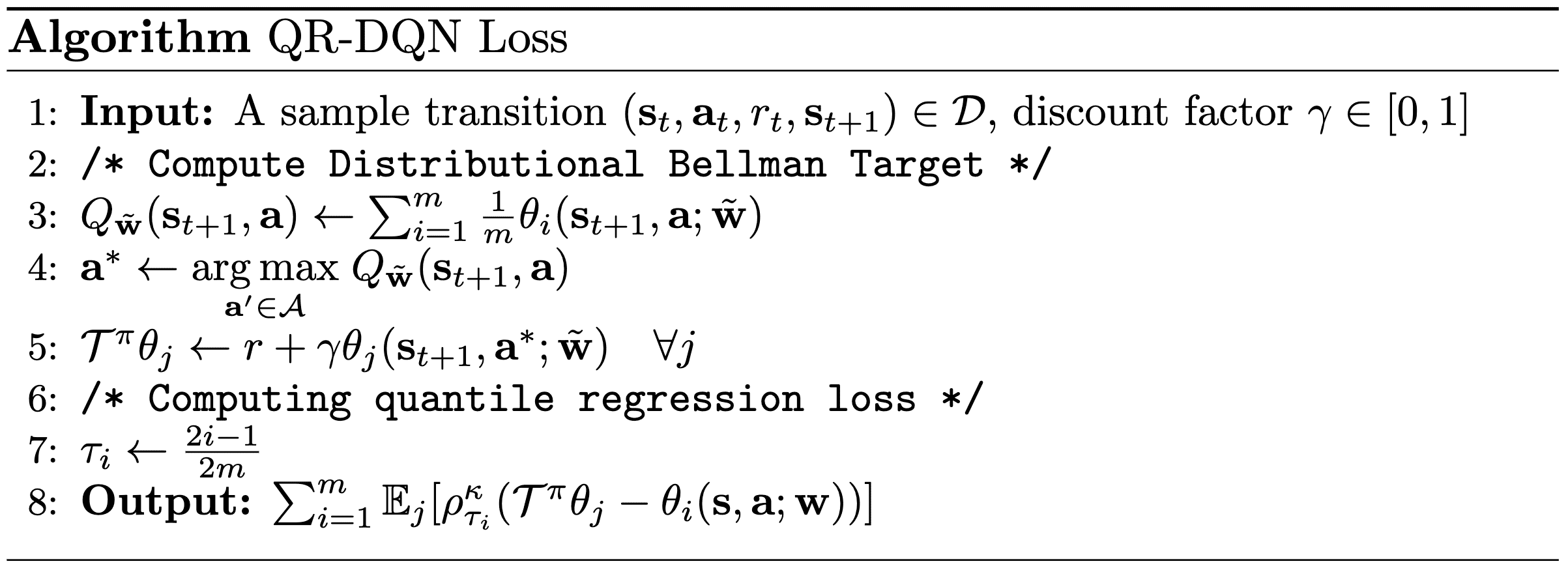
Consequently, QR-DQN outperforms all previous agents, including standard DQN, and C51, in mean and median human-normalized score on the Atari 2600 games.

$\mathbf{Fig\ 9.}$ Comparisons of QR-DQN (Dabney et al., AAAI 2018)

Implicit Quantile Network (IQN)

Implicit Parameterization

C51 and QR-DQN explicitly design the return distribution and are thus restricted to assigning probabilities to an a priori fixed, discrete set of possible return. In particular, the neural network of these algorithms take a state-action pair $(\mathbf{s}, \mathbf{a})$ as an input and outputs the distribution parameters such as the location $\theta$ or the softmax parameters $\varphi$.

Instead of designing the neural networks to represent the explicit distribution of $\eta$, we can consider implicit approach; by considering the return distribution function $\eta$ to be a mapping:

\[(\mathbf{s}, \mathbf{a}, \tau) \mapsto F_{\eta (\mathbf{s}, \mathbf{a})}^{-1} (\tau) \sim \eta (\mathbf{s}, \mathbf{a})\]

where $F_\nu^{-1}$ is the quantile function (inverse CDF) and $\tau \sim \mathcal{U} ([0, 1])$. The implicit quantile network (IQN) algorithm instantiates such principle by parameterizing the quantile function within the neural network.

• Advantages over QR-DQN
  • The approximation error is no longer governed by the number of quantiles of the network, but by the network’s size and the amount of training;
  • IQN can be used with a flexible number of samples per update, and thus improve data efficiency;
  • The implicit representation of the return distribution enables us to expand the class of policies to better leverage the learned distribution;

Preliminary: Risk-Sensitive RL

The objective of general RL problem is to find a optimal policy that maximizes the expected value of the return:

\[\mathcal{J}(\pi) = \mathbb{E} [ G (\mathbf{s}_0, \mathbf{a}_0) = \sum_{t=0}^\infty \gamma^t r(\mathbf{s}_t, \mathbf{a}_t)]\]

However, in practice, optimizing solely for the expected value may not be satisfactory due to variability from the tail of the return distribution. Therefore, it may be beneficial to incoporate the concept of variability into the optimization problem formulation. In this context, we refer to this variability as risk, and RL problem with risk-sensitivity is termed risk-sensitive RL.

Risk measure

The most prevalent approach to incorporate risk sensitivity into objective functions is to employ a risk measure $\rho$ that quantifies the level of risk. The fundamental concept is to transform the cumulative returns using appropriate risk measures and to seek optimal policies with respect to this measure:

\[\mathcal{J}_\rho (\pi) = \rho \left( \sum_{t=0}^\infty G (\mathbf{s}_0, \mathbf{a}_0 ) = \gamma^t r(\mathbf{s}_t, \mathbf{a}_t) \right)\]

For example, for parameters $\beta$ and $\tau \in (0, 1)$ that control the desired risk-sensitivity:

• Mean-Variance Risk: $\rho_{\texttt{MV}}^\beta (G) = \mathbb{E}[G] - \beta \mathrm{Var}(G)$
• Entropic Risk: $\rho_{\texttt{ER}}^\beta (G) = - \frac{1}{\beta} \log \mathbb{E}[e^{-\beta G}]$
• Value-at-risk (VaR): $\rho_{\texttt{VaR}}^\tau (G) = - F_{G}^{-1} (\tau)$ for $\tau \in (0, 1)$

Depending on the behavior of the objective, the objective is called risk-averse or risk-seeking. For instance, in mean-variance risk, it is risk-averse for $\beta > 0$ and risk-seeking for $\beta < 0$. The objective is called risk-neutral for $\beta = 0$, i.e., no risk-sensitivity is introduced.

Distortion risk measure

Among various measures, the risk measure related to the cumulative distribution function of the return (e.g., VaR) is termed a distortion risk measure, as it distorts the cumulative probabilities of the random variable. The distortion risk measure $\rho_\beta$ associated with the distortion measure $\beta: [0, 1] \to [0, 1]$ is mathematically defined as:

\[\rho_\beta (G) = \int_{-\infty}^\infty g \frac{\partial}{\partial g} \left( \beta \circ F_{G (\mathbf{s}, \mathbf{a})} \right) (g) \mathrm{d} g\]

For example, the following mappings are widely used for $\beta$:

• Cumulative Probability Weighting

\[\mathrm{CPW} (\eta, \tau) = \frac{\tau^\eta}{\left( \tau^\eta + (1-\tau)^\eta \right)^{\frac{1}{\eta}}}\]

• Power formula
  • Risk-averse for $\eta < 0$ and risk-seeking for $\eta > 0$

\[\mathrm{Pow} (\eta, \tau) = \begin{cases} \tau^{\frac{1}{1 + \vert \eta \vert}} & \quad \text{ if } \eta \geq 0 \\ 1 - ( 1 - \tau )^{\frac{1}{1 + \vert \eta \vert}} & \quad \text{ if } \eta < 0 \end{cases}\]

• Conditional Value-at-risk (CVaR)

\[\mathrm{CVaR} (\eta, \tau) = \eta \tau\]

Algorithm

The overall IQN algorithm is illustrated below compared to the DQN:

1. Prediction
   The IQN takes an input a tuple $(\mathbf{s}, \mathbf{a}, \tau)$. To make it easier for the neural network to work with the sample point $\tau \in (0, 1)$, $\tau$ is encoded to the $\mathbb{R}^M$-valued vector by the cosine embedding: $$ \varphi (\tau) = (\cos (\pi \tau i))_{i=0}^{M - 1} $$ and processed by fully-connected layer to generate the feature vector of $\tau$, denoted as $\phi (\tau)$: $$ \phi (\tau) = \texttt{ReLU}\left( \varphi (\tau) \cdot \mathbf{W} + \mathbf{b} \right) $$ And this feature of $\tau$ is combined with the state feature $\psi (\mathbf{s})$ that processed by another 3-layered fully-connected networks using Hadamard product $\odot$. Finally, the network outputs an $\vert \mathcal{A} \vert$-dimensional vector that approximates the evaluation of the quantile function $F_{\eta (\mathbf{s}, \mathbf{a})}^{-1} (\cdot)$ at this $\tau$: $$ \theta (\mathbf{s}, \mathbf{a}, \tau) = f( \psi(\mathbf{s}) \odot \phi(\tau) )_{\mathbf{a}} $$ where $f$ is a rectified linear transformation.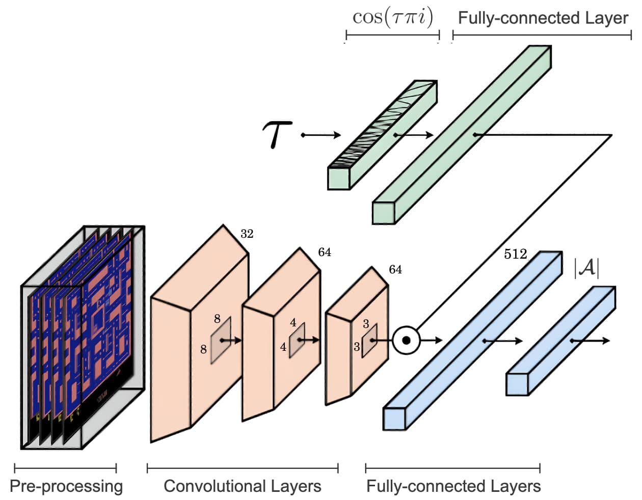

   

   $\mathbf{Fig\ 10.}$ The IQN Network (Bellemare et al., 2023)
   
   Since IQN represents the quantile function implicitly, the induced state-action value functions $Q_\mathbf{w}$ and target $Q_\tilde{\mathbf{w}}$ are approximated by a sampling procedure by uniform sampling $m$ i.i.d. levels $\tau_1, \cdots, \tau_m \sim \mathcal{U}(0, 1)$ and averaging the output of the network at these levels: $$ Q_\mathbf{w} (\mathbf{s}, \mathbf{a}) \approx \sum_{i=1}^m \frac{1}{m} \theta_\mathbf{w} (\mathbf{s}, \mathbf{a}, \tau_i) $$
2. Action
   The implicit representation of the return distribution enables the agents to broaden the class of policies to more effectively utilize the learned distribution. Observing that changing sample distribution for $\tau \sim \mathcal{U} (0, 1)$ is equivalent to evaluating $\tilde{\tau} \sim \beta (\mathcal{U} (0, 1))$ under a distortion risk measure $\beta: [0, 1] \to [0, 1]$: $$ Q (\mathbf{s}, \mathbf{a}) = \int_{-\infty}^\infty z \frac{\partial}{\partial z} F_{\eta (\mathbf{s}, \mathbf{a})} (z) \mathrm{d} z \implies Q_\beta (\mathbf{s}, \mathbf{a}) = \int_{-\infty}^\infty z \frac{\partial}{\partial z} (\beta \circ F_{\eta (\mathbf{s}, \mathbf{a})}) (z) \mathrm{d} z $$ the authors expanded the class of polices to $\varepsilon$-greedy on risk-sensitive policies with arbitrary distortion risk measures: $$ \pi_\beta (\mathbf{a}_t \vert \mathbf{s}_t) = \begin{cases} 1 & \quad \text{ if } \mathbf{a}_t = \underset{\mathbf{a} \in \mathcal{A}}{\arg \max} \; Q_{\mathbf{w}, \beta} (\mathbf{s}_t, \mathbf{a}) \\ 0 & \quad \text{ otherwise } \end{cases} $$ where $$ Q_{\mathbf{w}, \beta} (\mathbf{s}, \mathbf{a}) = \frac{1}{m} \sum_{i=1}^m \theta_\mathbf{w} (\mathbf{s}, \mathbf{a}, \tilde{\tau}_i) $$
   
   

   

   $\mathbf{Fig\ 11.}$ Effects of Risk-sensitive policies. (Dabney et al., 2018)
   
   
3. Learning
   Since the IQN takes state-action pair $(\mathbf{s}, \mathbf{a})$ with distribution level $\tau$ as an input, it first samples two levels $\tau, \tau^\prime \sim \mathcal{U}(0, 1)$. Then, from random transition $(\mathbf{s}, \mathbf{a}, r, \mathbf{s}^\prime) \sim \mathcal{D}$, the two-sample IQN loss is defined by: $$ \begin{gathered} \mathcal{L}_{\tau, \tau^\prime} (\mathbf{w}) = \rho_{\tau}^\kappa ( r + \gamma \theta_\tilde{\mathbf{w}} (\mathbf{s}^\prime, \mathbf{a}_{\tilde{\mathbf{w}}} (\mathbf{s}^\prime), \tau^\prime) - \theta_\mathbf{w} (\mathbf{s}, \mathbf{a}, \tau)) \\ \text{ where } \mathbf{a}_{\tilde{\mathbf{w}}} (\mathbf{s}^\prime) = \underset{\mathbf{a}^\prime \in \mathcal{A}}{\arg \max} \; Q_{\tilde{\mathbf{w}}, \beta} (\mathbf{s}^\prime, \mathbf{a}^\prime) \end{gathered} $$ Then, the IQN loss function is given by averaging the two-sample loss over many pairs of levels $\tau_1, \cdots, \tau_{m_1}$ and $\tau_1^\prime, \cdots, \tau_{m_2}^\prime$: $$ \mathcal{L}(\mathbf{w}) = \frac{1}{m_2} \sum_{i=1}^{m_1} \sum_{j=1}^{m_2} \mathcal{L}_{\tau_{i}, \tau_{j}^\prime} (\mathbf{w}) $$

The overall algorithm for computing the IQN loss is given by the following pseudocode:

$\mathbf{Fig\ 12.}$ The pseudocode for computing IQN loss.

And IQN demonstrated the greatest improvement over the previous state-of-the-art algorithms (QR-DQN and Rainbow).

$\mathbf{Fig\ 13.}$ Performances of IQN (Dabney et al., ICML 2018)

References

[1] Marc G. Bellemare and Will Dabney and Mark Rowland, “Distributional Reinforcement Learning”, MIT Press 2023
[2] Bellemare et al., “A Distributional Perspective on Reinforcement Learning”, ICML 2017
[3] Dabney et al., “Distributional Reinforcement Learning with Quantile Regression”, AAAI 2018
[4] Dabney et al., “Implicit Quantile Networks for Distributional Reinforcement Learning”, ICML 2018
[5] VITALab, “Distributional Reinforcement Learning with Quantile Regression”
[6] Wikipedia, “Distortion risk measure”