[RL] Imitation Learning with Behavior Cloning (BC)

Introduction

The goal of reinforcement learning is to optimize policies that maximize an accumulated reward, and in general it is assumed that the reward function is known or designed in prior. While successful in many settings, it also suffers from several challenges; determining an appropriate reward function for true purpose, sparse reward setting. Instead, the imitation learning approaches assume that the reward function is described implicitly through expert demonstrations. Given the expert policy \(\pi^*\), the imitation learning problem therefore aims to determine a policy $\pi_\theta$ that imitates the expert policy \(\pi^*\).

Behavior Cloning (BC)

A natural method is behavior cloning (BC), which reduces imitation learning to supervised learning.

Formulation

The simplest form of imitation learning might be to learn the expert’s policy using supervised learning. Simply, we can clone the expert by maximizing the probability of action taken for given observation:

\[\max_{\theta} \; \mathbb{E}_{\mathbf{o}_t \sim p_{\textrm{data}} (\mathbf{o}_t)} [\log \pi_{\theta} (\mathbf{a}_t \vert \mathbf{o}_t)]\]

However, we necessitate more precise measurement for the performance of the learned policy. Instead of just maximizing log probability, Behavior Cloning (BC) defines the cost function $c(\mathbf{s}_t, \mathbf{a}_t)$ and optimizes the policy by giving penalty if the student policy makes “mistake”:

\[\hat{\pi}^* = \underset{\theta}{\operatorname{argmin}} \; \mathbb{E}_{\mathbf{s}_t \sim p_{\textrm{data}} (\mathbf{s}_t) } [c(\mathbf{s}_t, \mathbf{a}_t)] \quad \text{ where } c \left(\mathbf{s}_t, \mathbf{a}_t\right) = \begin{cases} 0 & \quad \text { if } \mathbf{a}_t=\pi^* \left(\mathbf{s}_t\right) \\ 1 & \quad \text { otherwise } \end{cases}\]

Problem: Distributional Shift

The supervised learning approaches to RL (behaviour cloning) generally malfunction in the practical application since the training process is built upon the state samples provided by the expert, leading to distributional shift. The distributional mismatch is more likely in RL applications, since the i.i.d. assumptions that supervised learning postulates do not hold for the trajectory of the agent.

$\mathbf{Fig\ 1.}$ Distributional shift and compounding errors (Sergey Levine)

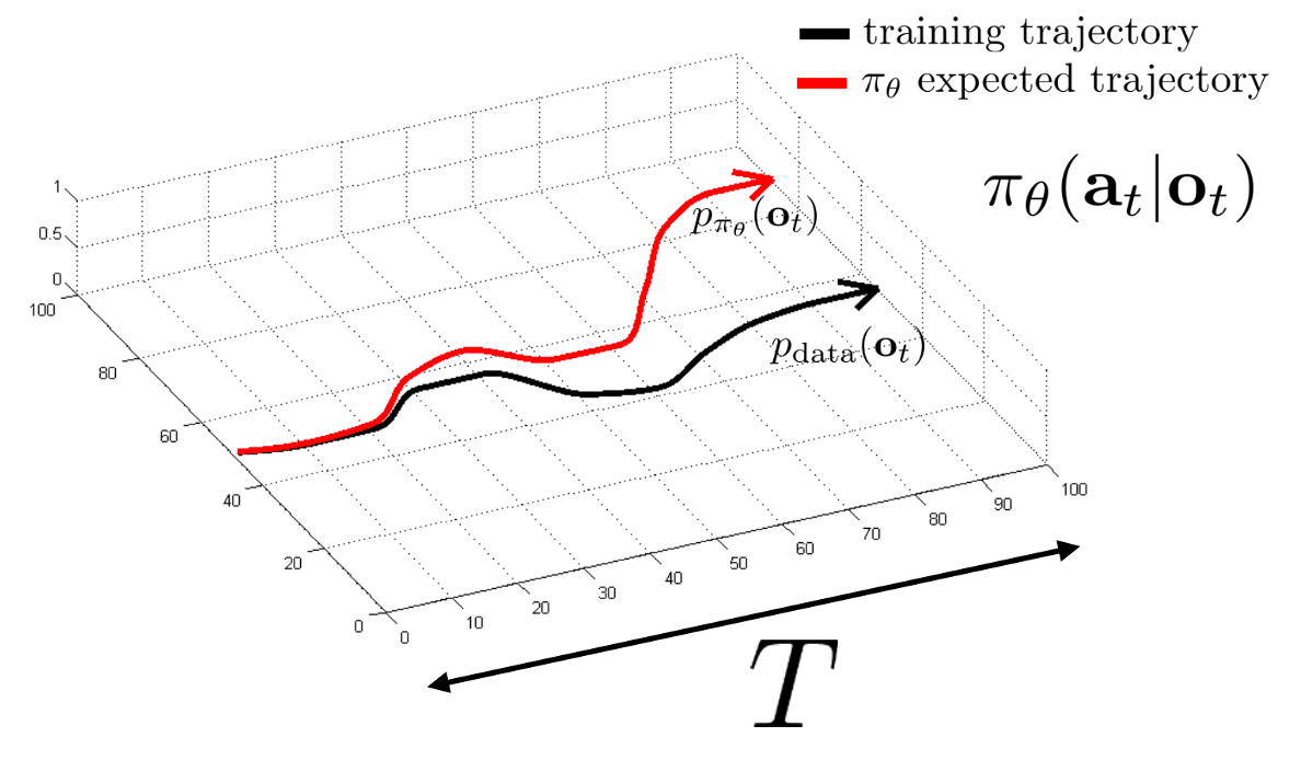
Intrinsically, supervised learning yields successful performance when training and test data distributions match. But in the formulation of reinforcement learning, the states derived from the expert policy \(\pi^*\) are not uniformly sampled throughout the entire state space. The learned policy $\pi_\theta$ produces its own distribution of states, thus it is prone to underperform when operating in states distant from the states encountered in the expert distributions. And the minor mistake of the learned agent may lead to severe degradations by compounding errors due to temporal structure in RL, thereby being a major challenge in imitation learning.

Error Bound

Following Ross and Bagnell, 2010, we can construct a simple upper-bound of the error occurred by distributional shift. Assume the loss function of imitation learning \(\ell (\mathbf{s}_t)\) to be $0-1$ loss of $\pi_\theta$ with respect to $\pi^*$:

\[\ell (\mathbf{s}_t) = \begin{cases} 0 & \text{ if } \pi_\theta (\mathbf{s}_t) = \pi^* (\mathbf{s}_t) \\ 1 & \text{ otherwise } \end{cases}\]

Denote the total loss of executing policy $\pi_\theta$ for $T$-steps as $\mathcal{J}(\pi_\theta)$:

\[\mathcal{J}(\pi_\theta) := \sum_{t=1}^T \mathbb{E}_{\color{red}{p_\theta (\mathbf{s}_t)}} [\ell (\mathbf{s}_t)]\]

where \(p_\theta (\mathbf{s}_t)\) is the average state distribution if we follow policy $\pi_\theta$ for $T$ steps. If we assume that the probability of making mistake in the dataset is less than $\epsilon$:

\[\mathbb{E}_{\color{blue}{p_{\pi^*} (\mathbf{s}_t)}} [\ell (\mathbf{s}_t)] = \mathbb{E}_{\color{blue}{p_\texttt{data} (\mathbf{s}_t)}} [\ell (\mathbf{s}_t)] \leq \epsilon\]

we can write \(p_\theta\) with respect to \(p_{\pi^*}\):

\[p_\theta (\mathbf{s}_t) = (1 - \epsilon)^t p_{\pi^*} (\mathbf{s}_t) + (1 - (1 - \epsilon)^t) p_\texttt{mistake} (\mathbf{s}_t)\]

By upper-bounding the sum of difference between \(p_{\pi^*}\) and \(p_\theta\) as follows:

\[\begin{aligned} \sum_{\mathbf{s}_t \in \mathcal{S}} \vert p_\theta (\mathbf{s}_t) - p_{\pi^*} (\mathbf{s}_t) \vert &= (1 - (1-\epsilon)^t) \sum_{\mathbf{s}_t \in \mathcal{S}} \vert p_{\texttt{mistake}} (\mathbf{s}_t) - p_{\pi^*} (\mathbf{s}_t) \vert \\ &\leq 2 (1 - (1-\epsilon)^t) \\ &\leq 2 \epsilon t \quad \because (1-\epsilon)^t \geq 1 - \epsilon t \text{ for } \epsilon \in [0, 1] \end{aligned}\]

we finally obtain the upper-bound of the distribution shift error with respect to the trajectory length $T$:

\[\begin{aligned} \mathcal{J}(\pi_\theta) & = \sum_{t=1}^T \sum_{\mathbf{s}_t \in \mathcal{S}} p_\theta (\mathbf{s_t}) \cdot \ell (\mathbf{s_t}) \\ & \leq \sum_{t=1}^T \sum_{\mathbf{s}_t \in \mathcal{S}} \left[ p_{\pi^*} (\mathbf{s}_t) \cdot \ell (\mathbf{s}_t) + \vert p_\theta (\mathbf{s}_t) - p_{\pi^*} (\mathbf{s}_t) \vert \cdot \ell_{\max} \right] \\ & \leq \sum_{t=1}^T \left[ \epsilon + 2 \epsilon t \right] \sim \mathcal{O}(\epsilon T^2) \end{aligned}\]

Therefore, $\pi_\theta$ trained by the traditional supervised learning approach has poor performance guarantees due to the quadratic growth in $T$.

DAgger: Dataset Aggregation

Formulation

The DAgger algorithm (Rose et al. AISTAT 2011) aims to provide a more principled solution to distributional shift problem of imitation learning, with the following simple idea:

Continually query domain expert to get more supervisions of the expert action along the trajectory taken by the learning policy $\pi_\theta$.

In other words, DAgger simply gathers new expert data as required. Whenever the learned policy $\pi_\theta$ navigates to states absent in the expert dataset, the agent just query the expert for additional information, thereby avoiding the errors from the distribution shift by matching the state distribution of data \(p_\texttt{data}(\mathbf{o}_t)\) to \(p_{\pi_\theta}(\mathbf{o}_t)\).

$\mathbf{Algorithm\ 1.}$ DAgger Algorithm (Rose et al. 2011)

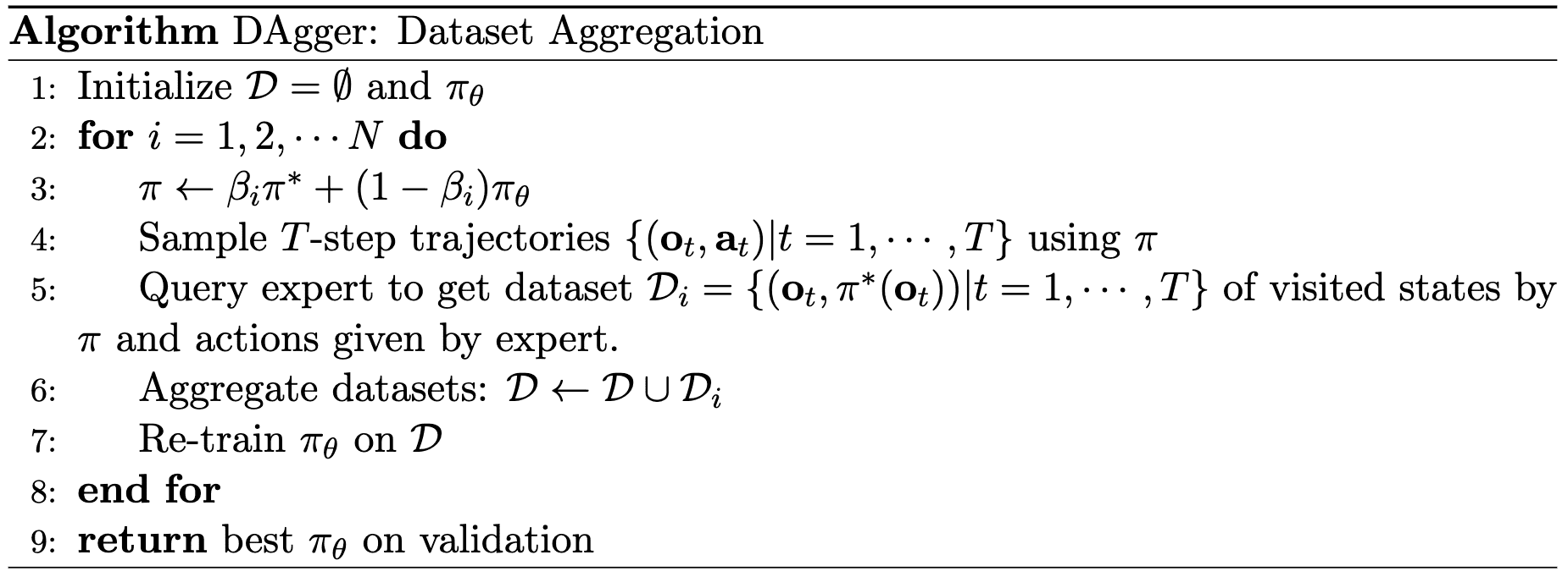
Here, $\beta_i$ is a pre-defined constant that converges to $0$ as $i \to \infty$. As time progresses, this iterative process guides the learned policy toward a more accurate approximation of the true policy, hence it diminishes the occurrence of distributional mismatch.

Limitation

A drawback to this approach is evident: at each step, the policy necessitates re-training, which can lead to computational inefficiencies. Furthermore, it is not intuitive to ask humans to evaluate the expert actions with single observation (and it is also daunting to us to label in real time). For instance, humans are generally situated on temporal process rather than making decisions instantaneously.

Theoretical Analysis

Recall that we derived that the performance $\mathcal{J} (\pi_\theta)$ of $\pi_\theta$ has $T$-quadratic upper-bound ($\mathcal{O} (\epsilon T^2)$). The authors demonstrated that the DAgger can be a room for better performance guarantee that is linear in $T$ under some conditions:

$\color{red}{\mathbf{Theorem.}}$ Performance Guarantee of DAgger
Denote $\pi_\theta$ at the $i$-th iteration as $\hat{\pi}_i$, true loss of the best policy as $\epsilon_N$: $$ \epsilon_N = \min_{\pi \in \Pi} \frac{1}{N} \sum_{i=1}^N \mathbb{E}_{\mathbf{s} \sim p_{\pi_i}} [ \ell (\mathbf{s}, \pi) ] $$ Assume that

• $\ell$ is strongly convex and bounded over $\Pi$;
• $\beta_i \leq (1 - \alpha)^{i - 1}$ for all $i$ for some constant $\alpha$ independent of $T$;
• The policy learning algorithm is no-regret algorithm that produces a sequence of policies $\{\pi_i\}_{i=1}^N$ such that the average regret with respect to the best policy goes to $0$ as $N$ goes to $\infty$: $$ \frac{1}{N} \sum_{i=1}^N \mathbb{E}_{\mathbf{s} \sim p_{\pi_i}} [\ell (\mathbf{s}, \pi_i)] - \min_{\pi \in \Pi} \frac{1}{N} \sum_{i=1}^N \mathbb{E}_{\mathbf{s} \sim p_{\pi_i}} [\ell (\mathbf{s}, \pi)] \leq \gamma_N $$ and $\gamma_N$ is $\tilde{\mathcal{O}}(\frac{1}{N})$

Then, in the infinite sample case (infinite number of sample trajectories at each iteration), if $N$ is $\tilde{\mathcal{O}}(T)$, there exists a policy $\hat{\pi} \in \{ \hat{\pi}_i \}_{i=1}^N$ such that: $$ \mathbb{E}_{\mathbf{s} \sim p_{\hat{\pi}}} [\ell (\mathbf{s}, \hat{\pi})] \leq \epsilon_N + \mathcal{O} \left( \frac{1}{T} \right) $$

$\mathbf{Proof.}$

Denote $\pi$ in the pseudocode at the $i$-th iteration as $\pi_i$. Let \(p_{\texttt{mistake}}\) be the state distribution over $T$ steps conditioned on $\pi_i$ selecting $\pi^*$ at least once over $T$ steps:

\[p_{\pi_i} (\mathbf{s}_T) = (1 - \beta_i)^T p_{\hat{\pi}_i} (\mathbf{s}_T) + (1 - (1 - \beta_i)^T) p_{\texttt{mistake}} (\mathbf{s}_T)\]

Similar to our theoretical discussion in the distribution shift, we can derive the following inequality:

\[\begin{aligned} \sum_{\mathbf{s}_T \in \mathcal{S}} \vert p_{\pi_i} (\mathbf{s}_T) - p_{\hat{\pi_i}} (\mathbf{s}_T) \vert &= (1 - (1-\beta_i)^T) \sum_{\mathbf{s}_T \in \mathcal{S}} \vert p_{\texttt{mistake}} (\mathbf{s}_T) - p_{\hat{\pi_i}} (\mathbf{s}_T) \vert \\ &\leq 2 (1 - (1-\beta_i)^T) \\ &\leq 2 \beta_i T \quad \because (1-\beta_i)^T \geq 1 - \beta_i T \text{ for } \beta_i \in [0, 1] \end{aligned}\]

Let $\ell_{\max}$ be an upper-bound on the loss $\ell$. The inequality above implies:

\[\mathbb{E}_{\mathbf{s} \sim p_{\hat{\pi}_i}} [\ell (\mathbf{s}, \hat{\pi}_i)] \leq \mathbb{E}_{\mathbf{s} \sim p_{\pi_i}} [\ell (\mathbf{s}, \hat{\pi}_i)] + 2 \ell_{\max} \min (1, T \beta_i)\]

Define $n_\beta$ to be the largest $n \leq N$ such that $\beta_n > \frac{1}{T}$.

\[\begin{aligned} \min_{\hat{\pi} \in \{ \hat{\pi}_i \}_{i=1}^N } \mathbb{E}_{\mathbf{s} \sim p_{\hat{\pi}}} [\ell (\mathbf{s}, \hat{\pi})] & \leq \frac{1}{N} \sum_{i=1}^N \mathbb{E}_{\mathbf{s} \sim p_{\hat{\pi}_i}} \\ & \leq \frac{1}{N} \sum_{i=1}^N \left( \mathbb{E}_{\mathbf{s} \sim p_{\pi_i}} [\ell (\mathbf{s}, \hat{\pi}_i)] + 2 \ell_{\max} \min (1, T \beta_i) \right)\\ & \leq \gamma_N + \frac{2 \ell_{\max}}{N} \left[ n_\beta + T \sum_{i=n_\beta + 1}^N \beta_i \right] + \min_{\pi \in \Pi} \sum_{i=1}^N \mathbb{E}_{\mathbf{s} \sim p_{\pi_i}} [\ell (\mathbf{s}, \pi)] \\ & = \gamma_N + \epsilon_N + \frac{2 \ell_{\max}}{N} \left[ n_\beta + T \sum_{i=n_\beta + 1}^N \beta_i \right] \end{aligned}\] \[\tag*{$\blacksquare$}\]

Other Challenges

Besides distributional shift, there are several long-standing obstacles for the imitation learning.

• Non-Markovian Behaviors
  Human decision-making is influenced by temporal context, challenging the imitation learning process that relies solely on current observations.
• Multimodal Behaviors
  Typically, there are few possible actions for the given observation, e.g. the agent can avoid the obstacle by moving either left or right.

Non-Markovian Behaviors

The majority of decisions made by humans are non-Markovian in nature: if we encounter the same situation twice, we are unlikely to respond in precisely the same manner based solely on the most recent time-step. The actions we take at present are influenced by events and experiences from previous time-steps, rendering training considerably more challenging.

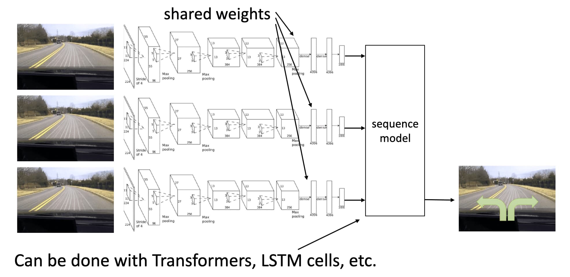
Sequence modeling with History

We can leverage the incorporation of historical information encoded by sequence models such as LSTMs or Transformers, instead of taking all the history of observations as input of the model.

$\mathbf{Fig\ 2.}$ Sequence Modeling (Sergey Levine)

Problem: Causal Confusion

The important caveat of leveraging history is causal confusion pointed by De Hann et al. NeurIPS 2019. To illustrate, consider behavioral cloning to train a neural network to drive a car (see $\mathbf{Fig\ 3.}$). In scenario A, the model is trained with an image including the dashboard, while in scenario B, the dashboard is masked out. Both models (with identical architecture) achieve low training loss, but during testing, model B performs well on the road while model A does not. The discrepancy arises because model A mistakenly associates the brake indicator light with braking, considering it as the cause rather than the effect, leading to poor performance despite low training error.

$\mathbf{Fig\ 3.}$ Causal misidentification: more information yields worse imitation learning performance. (De Haan et al. 2019)
Model A relies on the braking indicator to decide whether to brake. Model B instead correctly attends to the pedestrian

Multimodal Behaviors

Typically, the human behaviors are usually multi-modal; there are few possible actions for the given observation (e.g., the agent can avoid the obstacle by moving either left or right). And in a continuous action space, the MLE of the actions may be a problem if parametric distribution modeled for our policy is not multi-modal.

$\mathbf{Fig\ 4.}$ Multimodal Behavior (Sergey Levine)

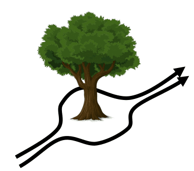
Most RL algorithms parameterize policies using deep neural networks with deterministic outputs or Gaussian distributions, thereby restricting learning to a single behavior mode. Training a policy with a single modality to maximize likelihood may result in it capturing the mean of two modes, potentially leading to unexpected situations (e.g., the agent may be trained to move directly towards an obstacle, representing the mean of moving left and right).

Expressive Continuous Distributions

One possible approach to learning expressive continuous distributions that capture multi-modality is through latent variable models. By designing the policy network with latent variable, the policy takes observation images and an additional latent variable as inputs, producing different modes of action distributions based on this latent variable.

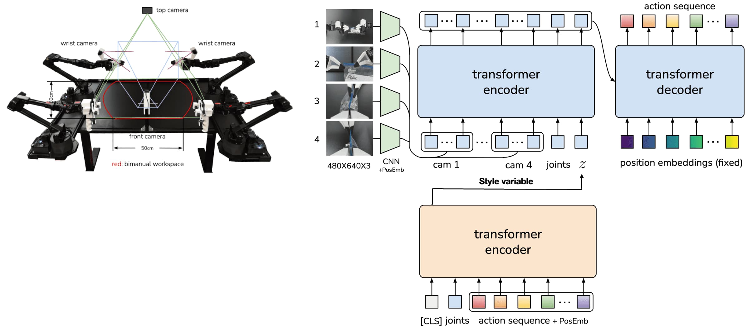
Action Chunking with Transformers (ACT) of Zhao et al., RSS 2023 trains the policy as a Conditional VAE (CVAE), which consists of an encoder and a decoder. The encoder of CVAE compresses the action sequence and joint observation into a style variable $z$, which accounts for the fact that human experts may perform tasks differently across trials. And the decoder (policy) of CVAE synthesizes images from multiple viewpoints, joint positions, and $z$ with Transformer-based architecture to predict a sequence of actions. At the test time, the encoder for $z$ is discarded and $z$ is simply set to the mean of the prior.

$\mathbf{Fig\ 5.}$ Architecture of Action Chunking with Transformers (Zhao et al., 2023)

The Diffusion model is also an effective approach that has recently demonstrated its expressiveness across various generation domains, including image and video. In light of the outstanding success of Diffusion, Chi et al., RSS 2023 proposed a Diffusion policy, which designs a robot’s visuomotor policy as a conditional denoising diffusion process. At time step $t$, the Diffusion policy takes the latest $T_\mathbf{o}$ steps of observation data \(\mathbf{o}_t\) as input and outputs $T_\mathbf{a}$ steps of actions \(\mathbf{a}_t\). To generate the action \(\mathbf{a}_t = \mathbf{a}_t^0\), it iterates through the following reverse diffusion process:

\[\begin{aligned} \mathbf{a}_t^{k - 1} & = \alpha ( \mathbf{a}_t^k - \beta \boldsymbol{\epsilon}_\theta (\mathbf{a}_t^k, \mathbf{o}_t, k) ) + \sigma_k \mathbf{z} \\ & \overset{\texttt{DDPM}}{=} \frac{1}{\sqrt{\alpha_k}} \left( \mathbf{a}_t^k - \frac{1 - \alpha_k}{\sqrt{1 - \bar{\alpha}_t}} \boldsymbol{\epsilon}_\theta (\mathbf{a}_t^k, \mathbf{o}_t, k) \right) + \sigma_k \mathbf{z} \end{aligned}\]

where $\mathbf{z} \sim \mathcal{N} (\mathbf{0}, \mathbf{I})$ is a white noise. And the authors demonstrated that the diffusion formulation offers significant advantages for robot policies, including the graceful handling of multimodal action distributions, suitability for high-dimensional action spaces, and its training stability.

$\mathbf{Fig\ 6.}$ Diffusion Policy (Chi et al., 2023)

Autoregressive Discretization

Discretization is another effective approach to learning a complex distribution that captures multi-modality. However, in higher dimensions, discretizing the full action space is impractical. Instead of predicting the discrete high-dimensional action all at once, we can represent the action distribution by factorizing it across dimensions:

\[p (\mathbf{a}_t \vert \mathbf{s}_t) = \prod_{i=1}^{d} p (a_{t, i} \vert \mathbf{s}_t, a_{t, 1:i-1}) \text{ where } \mathbf{a}_t = [a_{t, 1}, \cdots a_{t, d}]^\top \in \mathbb{R}^d\]

$\mathbf{Fig\ 7.}$ Autoregressive Discretization (Sergey Levine)

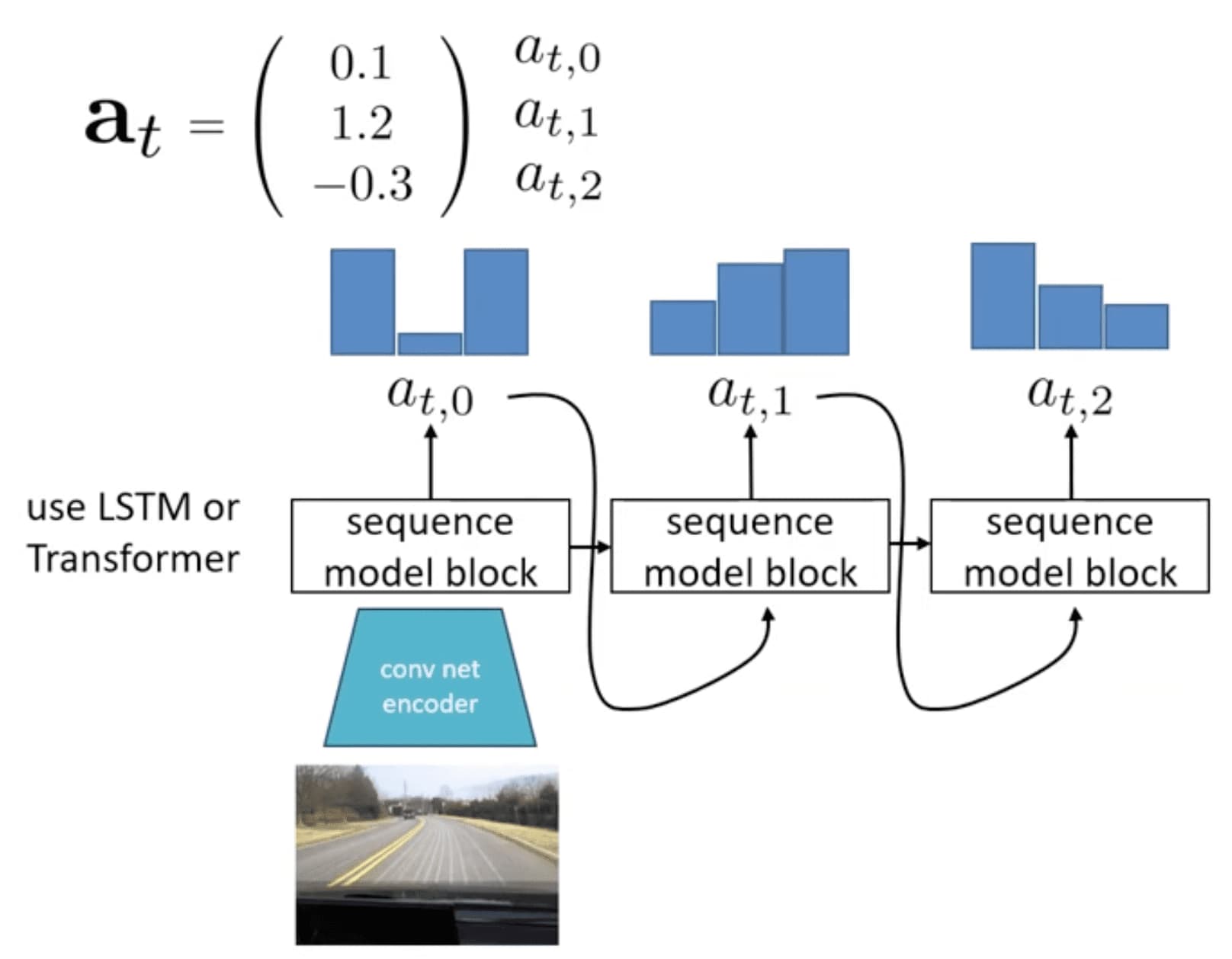
Robotics Transformer (RT-1) proposed by Brohan et al., RSS 2023 belongs to the autoregressive discretization category. This Transformer-based model processes a sequence of prior images and language instructions, and generates discrete, per-dimensional motion commands for the arm and base. Consequently, it frames the entire control problem as a sequence-to-sequence task. Due to the scalability of Transformer, RT-1 demonstrates robust generalization as a function of data size, model size, and data diversity, leveraging extensive data collected from real robots performing real-world tasks.

$\mathbf{Fig\ 8.}$ RT-1: Robotics Transformer (Brohan et al., 2023)

References

[1] CS 285 at UC Berkeley, “Deep Reinforcement Learning”
[2] Stanford CS 237B: Principles of Robot Autonomy II
[3] S. Ross and J. A. Bagnell., “Efficient reductions for imitation learning”, PMLR 2010
[4] Rose et al., “A Reduction of Imitation Learning and Structured Prediction to No-Regret Online Learning”, AISTAT2011
[5] De Haan et al., “Causal Confusion in Imitation Learning”, NeurIPS 2019
[6] Chi et al., “Diffusion Policy: Visuomotor Policy Learning via Action Diffusion”, RSS 2023
[7] Zhao et al., “Learning Fine-Grained Bimanual Manipulation with Low-Cost Hardware”, RSS 2023
[8] Brohan et al., “RT-1: Robotics Transformer”, RSS 2023