[RL] Deep Q-Learning: DQN Extensions
Success of deep Q-learning, especially DQN in the Atari, has led to huge excitement in using deep neural networks to do value function approximation in RL. Some immediate improvements include double DQN (Van Hasselt et al., AAAI 2016), prioritized replay (Schaul et al., ICLR 2016), Dueling DQN (Wang et al., ICML 2016), and NoisyNet (Fortunato et al., ICLR 2018). And Rainbow DQN (Hessel et al., AAAI 2018) combined these improvements into one algorithm, demonstrating the state-of-the-art performance on the Atari benchmark. This post provides the brief overview of these DQN-based algorithms.
Double DQN (DDQN)
Motivation: Overoptimism of Q-Learning
Recall the update rule of Q-learning with estimated state-action value $Q$:
\[Q(\mathbf{s}, \mathbf{a}) \leftarrow Q(\mathbf{s}, \mathbf{a}) + \alpha \left[ r(\mathbf{s}, \mathbf{a}) + \gamma \underset{\mathbf{a}^\prime \in \mathcal{A}}{\max} Q (\mathbf{s}^\prime, \mathbf{a}^\prime) - Q(\mathbf{s}, \mathbf{a}) \right]\]While this update will asymptotically approach the true optimal Q-value when $Q( \mathbf{s}, \mathbf{a})$ aligns with the true Q-value, it remains merely an estimation of the true Q-value. Consequently, the presence of noise in this estimation could impede the algorithm’s convergence to the true value. Indeed, Q-learning is known to incur a maximization bias-often referred to as overoptimism-the overestimation of the maximum expected action value. This issue was initially investigated by Thrun and Schwartz, 1993, wherein they theoretically demonstrated that if the action values contain random errors uniformly distributed in $[−\varepsilon, \varepsilon]$ then each target is overestimated up to $\gamma \varepsilon \frac{m−1}{m + 1}$ where $m$ is the number of actions.
The devil is in the $\max$ operator
The fundamental reason of the phenomenon lies in the $\max$ operator in the $Q$ target. As a consequence of function approximation noise, certain Q-values might be too small, while others might be excessively large. The $\max$ operator, however, always selects the largest value, rendering it especially sensitive to overestimations.
\[\underbrace{\mathbb{E} [\max ( Q_1, Q_2 )]}_{\text{What we are using}} \geq \underbrace{\max (\mathbb{E} [Q_1], \mathbb{E} [Q_2])}_{\text{What we want}}\]To provide an intuitive understanding, consider the following example, borrowed from Ameet Deshpande’s post:
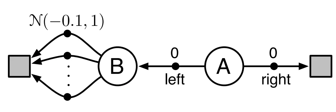
Suppose that the agent initially resides in state $\textrm{A}$ and if it selects the action $\textrm{right}$, it transitions to a terminal state and receives a reward of $0$. Conversely, if it selects the action $\textrm{left}$, it moves to state $\textrm{B}$, from which there exist numerous actions, each yielding rewards sampled from the Gaussian $\mathcal{N}(-0.1, 1)$, resulting in an expected reward of $-0.1$. In expectation, selecting the action $\textrm{right}$ appears advantageous due to the higher expected reward of $0$. However, the presence of reward variance gives rise to an unforeseen outcome.
Consider the scenario wherein the agent transitions to state $\textrm{B}$ and iteratively updates $Q$ by undergoing three trials, with two distinct actions $\mathbf{a}_1$ and $\mathbf{a}_2$ available at state $\textrm{B}$ for each trial, as outlined below:
As depicted in the table, despite $Q(\textrm{B}, \mathbf{a}_1)$ and $Q(\textrm{B}, \mathbf{a}_2)$ displaying negative values, the agent persistently chooses the $\textrm{left}$ action at state $\textrm{A}$. This behavior arises because the $\max$ operator exclusively neglect the negative value and optimistically selects the largest value.
Double Q-Learning
Therefore, the max operator in standard Q-learning (and DQN) uses the identical values both for action selection and evaluation, thus increasing the likelihood of selecting overestimated values and yielding overly optimistic value estimates. To mitigate this issue, we can simply decouple the selection from the evaluation, and such an approach is referred to as double Q-Learning proposed by [ 2010]. In double Q-Learning, two different Q-values $Q^A ( \cdot ; \boldsymbol{\theta}_A)$ and $Q^B ( \cdot ; \boldsymbol{\theta}_B)$ are learned by assigning each experience randomly to update one of the two Q-value functions. Consequently, the agent disentangles the selection and evaluation processes in Q-learning and revises its target as follows:
\[r (\mathbf{s}, \mathbf{a}) + \gamma \cdot Q (\mathbf{s}^\prime, \underset{\mathbf{a}^\prime \in \mathcal{A}}{\operatorname{arg max}} Q (\mathbf{s}^\prime, \mathbf{a}^\prime; \boldsymbol{\theta}); \boldsymbol{\theta}^\prime)\]In this formulation, $Q^A$ is utilized for action selection, while $Q^B$ evaluates the chosen action with the Q target. And the roles of the two Q functions are randomly interchanged, as delineated in the following pseudocode:
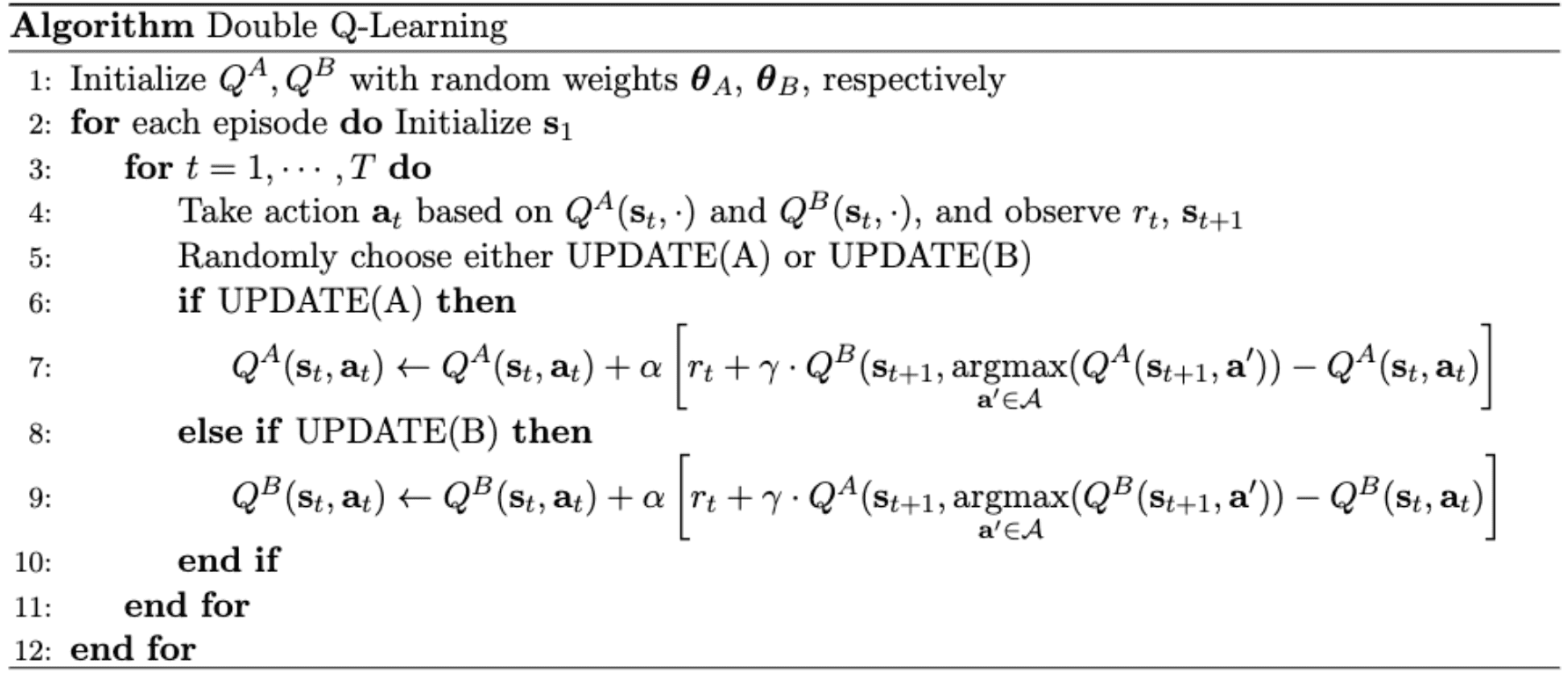
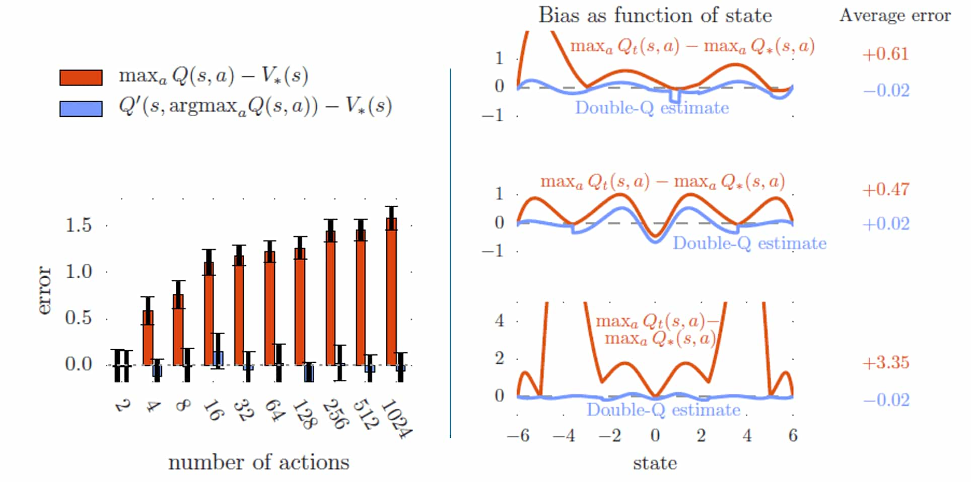
Consequently, double Q-learning is much robust to the overestimation regardless of the dimension of action space, while the overoptimism of the standard Q-learning increases with the number of actions as shown in the left part of figure below:
Double Deep Q-Network
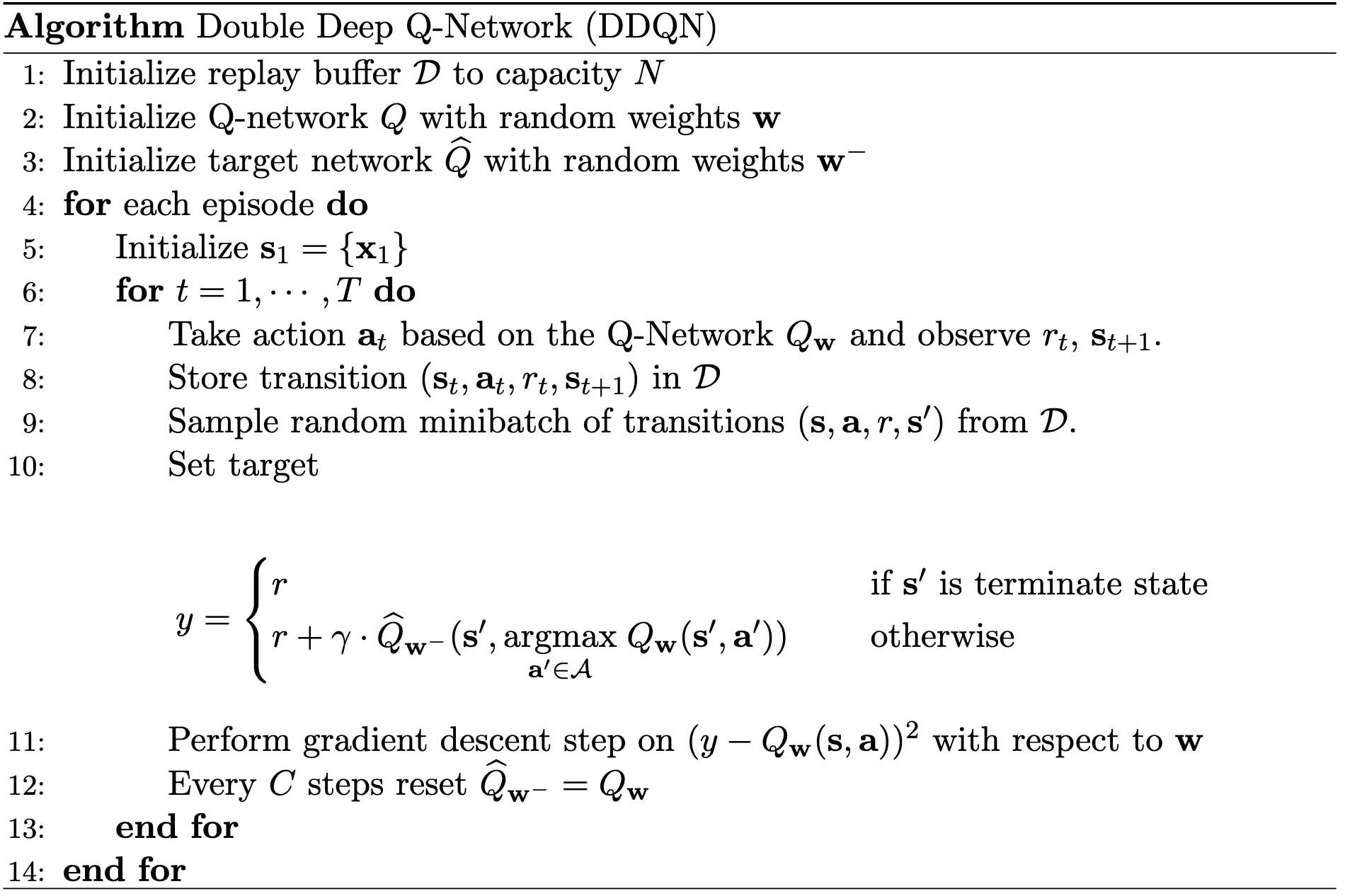
Double Deep Q-Network (DDQN) is the combination of the idea of Double Q-learning and DQN. Naturally, the Q-network \(Q_\mathbf{w}\) selects the action for the maximal value of the next state, while the target network \(\widehat{Q}_{\mathbf{w}^-}\) evaluate the action value:
\[\begin{array}{rlr} r (\mathbf{s}, \mathbf{a}) + \gamma \cdot \color{red}{\widehat{Q}_{\mathbf{w}^-} ( \mathbf{s}^\prime, \underset{\mathbf{a}^\prime \in \mathcal{A}}{\operatorname{arg max}} \; Q_\mathbf{w} (\mathbf{s}^\prime, \mathbf{a}^\prime))} & \textrm { (Double DQN) } \\ r (\mathbf{s}, \mathbf{a}) + \gamma \cdot \color{blue}{\underset{\mathbf{a}^\prime \in \mathcal{A}}{\max} \; \widehat{Q}_{\mathbf{w}^-} ( \mathbf{s}^\prime, \mathbf{a}^\prime)} & \textrm { (Standard DQN) } \\ \end{array}\]where the gradient for learning Q-network is thus given by
\[\nabla \mathbf{w} = \alpha \times \left[ r (\mathbf{s}, \mathbf{a}) + \gamma \cdot \widehat{Q}_{\mathbf{w}^-} ( \mathbf{s}^\prime, \underset{\mathbf{a}^\prime \in \mathcal{A}}{\operatorname{arg max}} \; Q_\mathbf{w} (\mathbf{s}^\prime, \mathbf{a}^\prime)) - Q_\mathbf{w} (\mathbf{s}, \mathbf{a}) \right] \times \nabla_{\mathbf{w}} Q_\mathbf{w} (\mathbf{s}, \mathbf{a}).\]
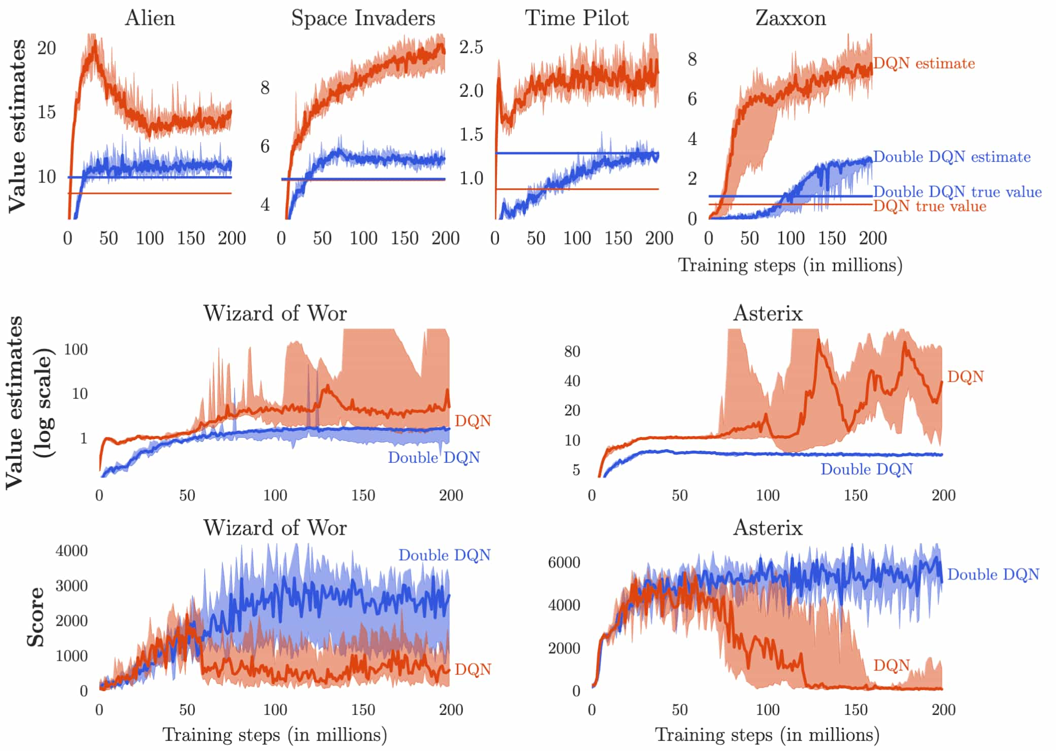
$\mathbf{Fig\ 5.}$ illustrates instances of overestimations across 6 Atari games and the adverse impact on the agent’s achieved scores during training. The scores decline when the overestimations begin. DQN consistently exhibits significant overoptimism regarding the value of the current greedy policy, while the learning curves for Double DQN, depicted in blue, closely align with the blue straight line representing the true value of the final policy. This suggests that Double DQN not only generates more precise value estimates but also yields better policies than DQN.
Aside: Prioritized Experience Replay (PER)
An advancement in experience replay called prioritized experience replay (PER), introduced in Schaul et al., 2016, extended the capabilities of DDQN and achieved further enhancements in the state-of-the-art. The core idea of the PER is to increase the replay probability of pivotal experience tuples that are more significant, informative, or task-relevant. And this quantity is measured through the proxy of absolute TD-error. Consequently, this approach facilitated accelerated learning and improved learned policy quality across the majority of games within the Atari benchmark, surpassing the performance of uniform experience replay.
Stochastic Prioritization
Let $i$ be the index of the $i$-th tuple of experience \((\mathbf{s}_i, \mathbf{a}_i, r_i, \mathbf{s}_{i+1})\). We sample tuples for update using priority function. The priority of a tuple $i$, denoted as $p_i$, is proportional to DQN error:
\[p_i = \left\vert r_i + \gamma \cdot \underset{\mathbf{a}^\prime \in \mathcal{A}}{\max} \; \widehat{Q}_{\mathbf{w}^-} (\mathbf{s}_{i+1}, \mathbf{a}^\prime) - Q_{\mathbf{w}} (\mathbf{s}_i, \mathbf{a}_i) \right\vert = \lvert \delta_i \rvert\]To obtain the robustness from the noise and the diversity of replay, instead of selecting the maximal prioritized tuple (called greedy TD-error prioritization) we adopt the stochastic sampling method that interpolates between pure greedy prioritization and uniform random sampling. We define the probability of selecting the $i$-th tuple as
\[\mathbb{P}(i) = \frac{p_i^\alpha}{\sum_{k} p_k^\alpha}\]where $\alpha$ is a hyperparameter that determines how much prioritization is used; note that $\alpha = 0$ corresponds to the general uniform case.
Other variants of computing $p_i$ are also possible:
-
proportional prioritization: $p_i = \lvert \delta_i \rvert + \varepsilon$
- where $\varepsilon$ is a small positive constant that prevents the edge-case of transitions not being revisited once their error is zero
-
rank-based prioritization: $p_i = (\textrm{rank}(i))^{-1}$
- where $\textrm{rank}(i)$ is the rank of transition $i$ when the replay memory is sorted according to TD error $\lvert \delta_i \rvert$.
Importance Sampling
Prioritized replay introduces bias because it changes the training distribution in an uncontrolled fashion. We can correct this bias by using importance-sampling (IS) weights. The weights are given by
\[w_i = \left(\frac{1}{N} \times \frac{1}{\mathbb{P}(i)} \right)^\beta\]where $\beta$ is a hyperparameter that determines how much correction is used:
- $\beta = 0$: no bias correction;
- $\beta = 1$: no priority (uniform);
These weights are folded into the Q-learning update by using $\frac{w_i}{\max_j w_j} \delta_i$ instead of the standard TD error $\delta_i$ where we normalize weights by $1/\max_i w_i$ for stability:
\[\begin{aligned} & \texttt{DQN:} \quad \boldsymbol{\theta} \leftarrow \boldsymbol{\theta} - \eta \cdot \delta_i \cdot \nabla_{\boldsymbol{\theta}} Q_\boldsymbol{\theta} (\mathbf{s}_i, \mathbf{a}_i) \\ & \texttt{PER:} \quad \boldsymbol{\theta} - \eta \cdot \color{red}{\frac{w_i}{\max_j w_j}} \cdot \delta_i \cdot \nabla_{\boldsymbol{\theta}} Q_\boldsymbol{\theta} (\mathbf{s}_i, \mathbf{a}_i) \end{aligned}\]Dueling DQN
Dueling Architecture
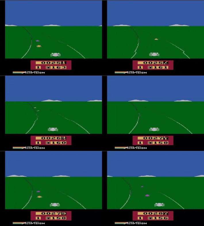
In certain applications, estimating the value of each action choice for numerous states may be unnecessary. While it’s crucial to determine the optimal action in some states, in many others, the choice of action holds little significance. For instance, in the Enduro game setting, deciding whether to move left or right only becomes consequential when a collision is obvious.
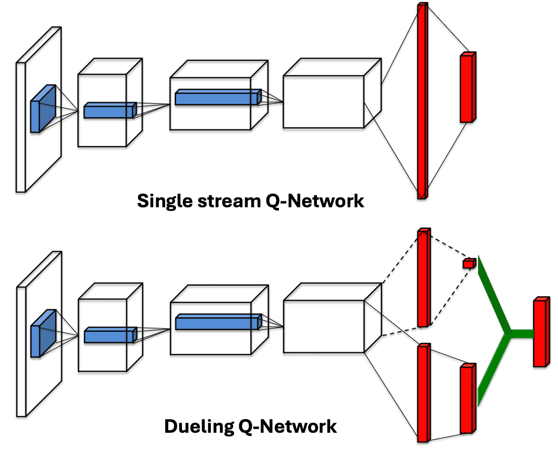
From the understanding that Q-value function $Q^\pi (\mathbf{s}, \mathbf{a})$ can be derived by summing the advantage function $A^\pi (\mathbf{s}, \mathbf{a})$ and the state-value function $V^\pi (\mathbf{s})$, Wang et al., ICML 2016 introduced the dueling architecture. This architecture explicitly segregates the representation of state-values and state-dependent action advantages via two distinct streams of fully-connected layers as illustrated in $\mathbf{Fig\ 7}$. Instead of employing a single sequence of fully connected layers following the convolutional layers, it employs two streams of fully-connected layers. These streams are designed to provide separate estimations of the value and advantage functions. Subsequently, the two streams are combined to generate a single Q-value.
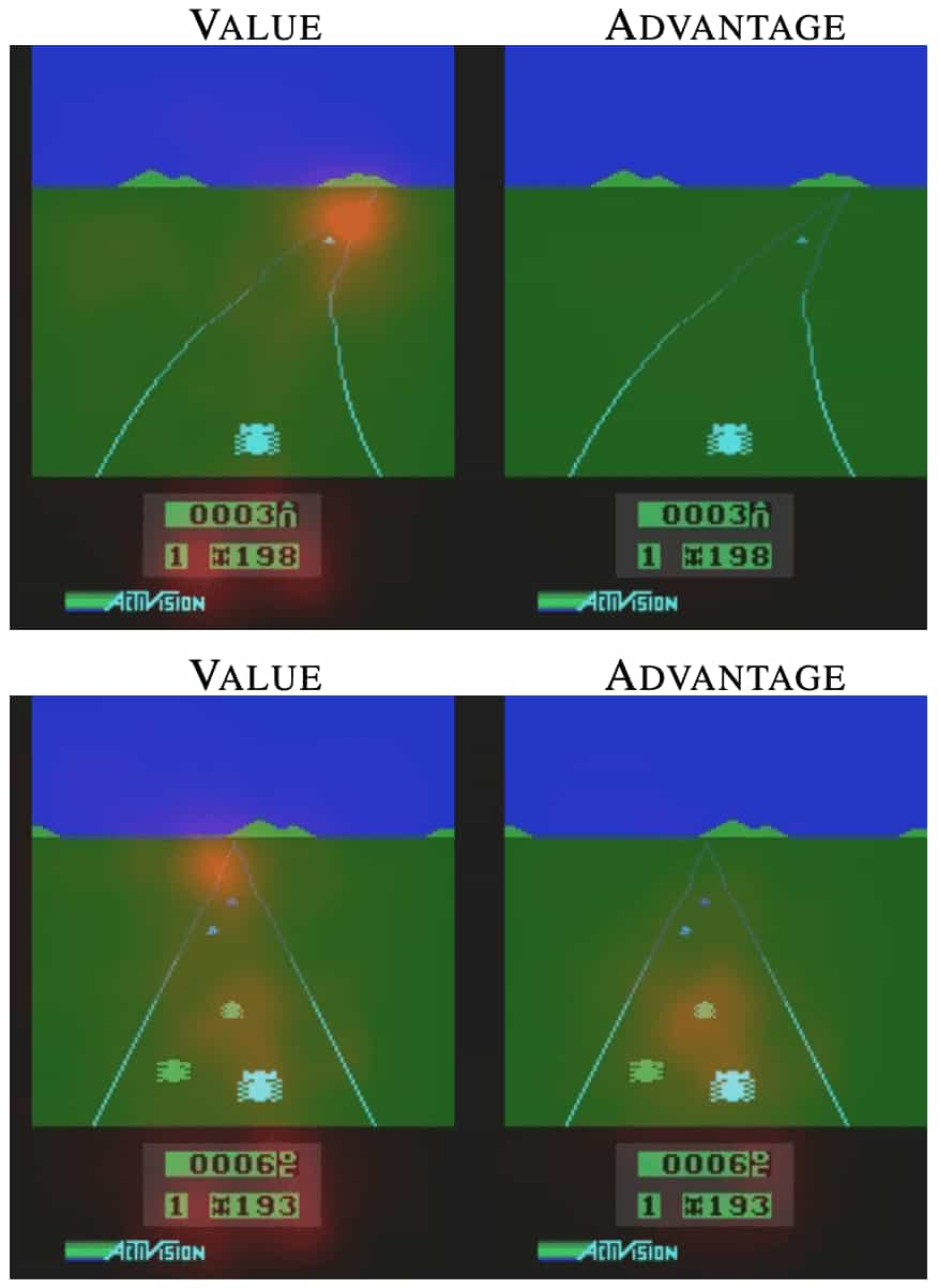
Intuitively, by decoupling the estimation of state-value and the assessment of the importance of each action at a given state, the agents is now capable of evaluating which states are (or are not) valuable, without needing to learn the effect of each action at each state. For instance, in the Enduro environment illustrated below, the value stream learns to pay attention to the road, while the advantage stream does not pay much attention to the typical visual input but does pay attention only when there are cars immediately in front, aiming to avoid collisions.
Dueling Q-Learning
Now, we need to aggregate the state-value function and advantage function for Q-learning. As an initial step, it is straightforward to obtain the Q function as the sum of state value function and advantage function:
\[Q_{\mathbf{w}, \alpha, \beta} (\mathbf{s}, \mathbf{a}) = V_{\mathbf{w}, \alpha} (\mathbf{s}) + A_{\mathbf{w}, \beta} (\mathbf{s}, \mathbf{a})\]where $\alpha$ and $\beta$ are the parameters of the two streams of fully connected layers and $\mathbf{w}$ denotes the parameters of the convolutional layers. However, this equation is unidentifiable in the sense that given $Q$ we cannot recover $V$ and $A$ uniquely. (For example, $Q = V + A = (V + c) + (A - c)$.)
To address this identifiability issue, from the Bellman optimality equations \(Q^* (\mathbf{s}, \mathbf{a}^*) = V^* {\mathbf{s}}\), we can force the advantage function estimator to have zero advantage at the chosen action:
\[Q_{\mathbf{w}, \alpha, \beta} (\mathbf{s}, \mathbf{a}) = V_{\mathbf{w}, \alpha} (\mathbf{s}) + \left( A_{\mathbf{w}, \beta} (\mathbf{s}, \mathbf{a}) - \underset{\mathbf{a}^\prime \in \mathcal{A}}{\max} A_{\mathbf{w}, \beta} (\mathbf{s}, \mathbf{a}^\prime) \right)\]Now for \(\mathbf{a}^* = \textrm{arg max}_{\mathbf{a}^\prime \in \mathcal{A}} Q_{\mathbf{w}, \alpha, \beta} (\mathbf{s}, \mathbf{a}^\prime)\), we obtain $Q_{\mathbf{w}, \alpha, \beta} (\mathbf{s}, \mathbf{a}^*) = V_{\mathbf{w}, \alpha} (\mathbf{s})$. An alternative aggregation module is suggested by replacing the max operator with an average, as shown in the figure below:
\[Q_{\mathbf{w}, \alpha, \beta} (\mathbf{s}, \mathbf{a}) = V_{\mathbf{w}, \alpha} (\mathbf{s}) + \left( A_{\mathbf{w}, \beta} (\mathbf{s}, \mathbf{a}) - \frac{1}{\vert \mathcal{A} \vert}\sum_{\mathbf{a}^\prime \in \mathcal{A}} A_{\mathbf{w}, \beta} (\mathbf{s}, \mathbf{a}^\prime) \right)\]

The average aggregation loses the original meaning of $V$ and $A$ because they are now off-target by a constant. Nevertheless, it enhances the stability of the optimization since the advantages only need to adapt as fast as the mean of the entire action space, ratherthan having to compensate any change to the optimal action’s advantage, which can vary from each state and training step. It’s important to note that subtracting the mean aids in identifiability without altering the relative ranking of the $A$ values. This preservation ensures that any greedy or $\epsilon$-greedy policy based on Q-values remains unchanged.
Also, our modification is viewed and implemented as part of the network and not as a separate algorithmic step, hence we don’t need to modify our pseudocode of DQN except the design of neural networks.
Aside: Noisy Network
Although a plethora of research is dedicated to efficient methods for exploration, most exploration heuristics in deep RL rely on random perturbations of the agent’s policy such as $\varepsilon$-greedy and entropy regularization due to its simplicity. Fortunato et al., 2018 proposed a simple approach called NoisyNet that applies random perturbations to the network weights.
The key insight is that a single modification to the weight vector can induce a consistent and potentially complex, state-dependent change in policy across multiple time steps—unlike dithering approaches where uncorrelated (and, in the case of $\varepsilon$-greedy, state-independent) noise is introduced to the policy at each step. For a linear layer of a neural network:
\[\boldsymbol{y} = \boldsymbol{w} \boldsymbol{x} + \boldsymbol{b}\]where $\boldsymbol{x} \in \mathbb{R}^p$ is the input vector, $\boldsymbol{w} \in \mathbb{R}^{q \times p}$ is the weight and $\boldsymbol{b} \in \mathbb{R}^q$ bias, the corresponding noisy linear layer is defined as:
\[\boldsymbol{y} = (\boldsymbol{\mu^w} + \boldsymbol{\Sigma^w} \odot \boldsymbol{\varepsilon^w}) \boldsymbol{x} + (\boldsymbol{\mu^b} + \boldsymbol{\Sigma^b} \odot \boldsymbol{\varepsilon^b})\]where $\boldsymbol{\varepsilon} \sim \mathcal{N}(\mathbf{0}, \mathbf{I})$, and $(\boldsymbol{\mu}, \Sigma)$ are learnable parameters.
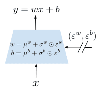
For random perturbations, two options are possible:
- Independent Gaussian noise
We can simply use an independent Gaussian noise entry per weight: $$ \{ \varepsilon_{i, j}^\boldsymbol{w}, \varepsilon_{k}^\boldsymbol{b} \vert 1 \leq i, k \leq q, 1 \leq j \leq p \} \overset{\textrm{i.i.d.}}{\sim} \mathcal{N}(0, 1) $$ therefore $pq + q$ noise variables. - Factorized Gaussian noise
To reduce the computation time of random sampling, we can use an independent noise per each output and another independent noise per each input. Specifically, draw $p$ unit Gaussian variables $\varepsilon_i$ for input dimension and $q$ unit Gaussian variables $\varepsilon_j$ for output dimension: $$ \{ \varepsilon_i, \varepsilon_j \vert 1 \leq i \leq p, 1 \leq j \leq q \} \overset{\textrm{i.i.d.}}{\sim} \mathcal{N}(0, 1) $$ yielding: $$ \begin{aligned} \varepsilon_{i, j}^\boldsymbol{w} & = f(\varepsilon_i) f(\varepsilon_j) \\ \varepsilon_j^\boldsymbol{b} & = f(\varepsilon_j) \end{aligned} $$ where $f: \mathbb{R} \to \mathbb{R}$. In the paper, $f(x) = \mathrm{sgn}(x) \sqrt{\vert x \vert}$.
And the NoisyNet parameters $(\mu, \Sigma)$ are optimized concurrently with the loss $\mathcal{L}$ of the RL problem during training.
Rainbow DQN
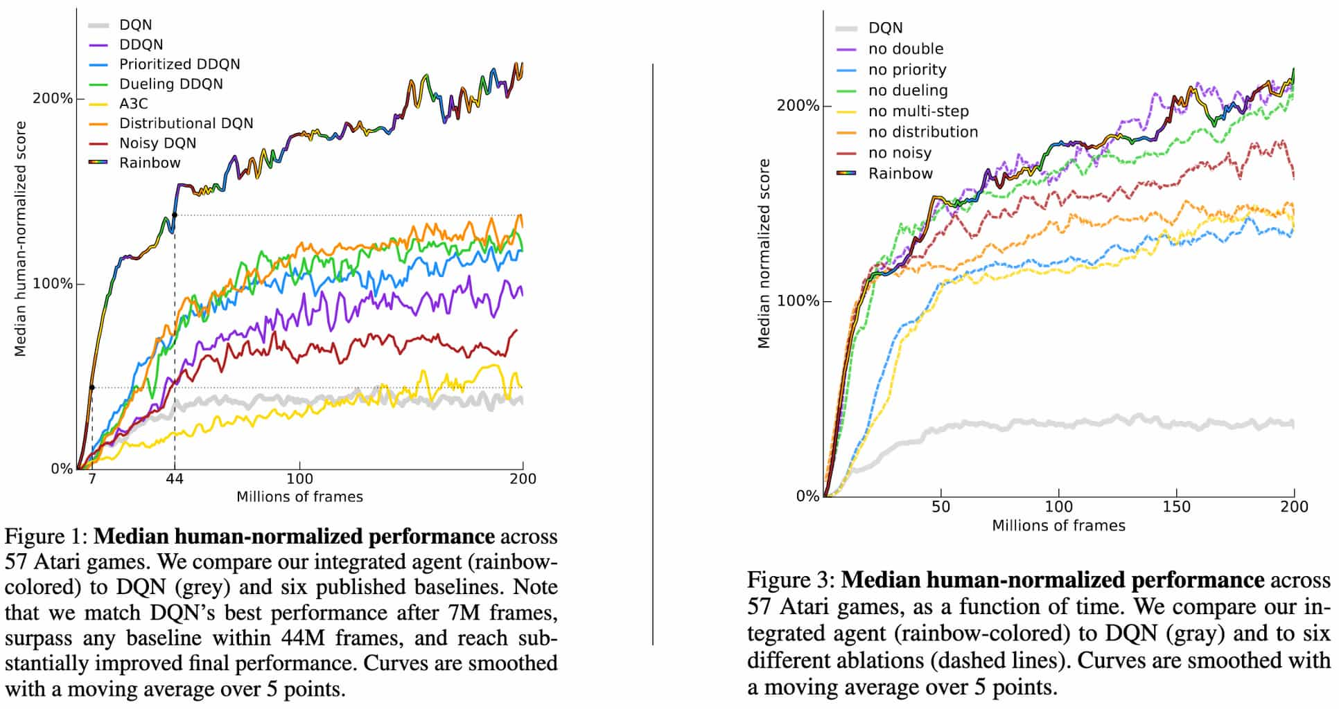
By integrating all the following components into a single integrated agent:
- Decoupling selection and evaluation of the bootstrap action (Double Q-Learning);
- Prioritized experience replay (PER);
- Multi-step bootstrap targets (A3C);
- Dueling network architecture (Dueling DQN);
- Estimating a categorical distribution of returns (C51);
- Stochastic linear layers (NoisyNet);
Rainbow demonstrated the state-of-the-art performance on the Atari 2600 benchmark, both in terms of data efficiency and final performance.
- Multi-step distribution loss
Let $R_t^{(n)}$ denote the $n$-step return, which is defined as: $$ R_t^{(n)} = \sum_{k=0}^{n - 1} \gamma \gamma_t^{(k)} R_{t + k + 1} $$ For a vector $\boldsymbol{z}$ of $N_{\textrm{atoms}}$ atoms that defines the support of categorical distribution: $$ z^i = v_{\min} + (i - 1) \frac{v_{\max} - v_{\min}}{N_{\textrm{atoms}} - 1} \text{ for } i \in \{ 1, \cdots, N_{\textrm{atoms}} \} $$ the $n$-step target categorical distribution is defined by target network with Double Q-Learning framework as follows: $$ \begin{gathered} d_t^{(n)} = (R_t^{(n)} + \gamma_t^{(n)} \boldsymbol{z}, \boldsymbol{p}_{\tilde{\mathbf{w}}} (\mathbf{s}_{t+n}, \mathbf{a}_{t+n}^*) ) \\ \text{ where } \mathbf{a}_{t+n}^* = \underset{\mathbf{a}^\prime \in \mathcal{A}}{\arg \max} \; Q_\mathbf{w} (\mathbf{s}_{t+n}, \mathbf{a}^\prime) \end{gathered} $$ This is approximated by the Q-network that produces the categorical distribution: $$ d_t = (\boldsymbol{z}, \boldsymbol{p}_\mathbf{w} (\mathbf{s}_t, \mathbf{a}_t)) $$ by $n$-step variant of the C51 loss: $$ \mathrm{KL} ( \Pi_\boldsymbol{z} d_t^{(n)} \Vert d_t ) $$ where $\Pi_\boldsymbol{z}$ is the projection onto $\boldsymbol{z}$. - KL-prioritization
Since the algorithm is minimizing the KL loss, PER is operated by KL-prioritizations instead of the absolute TD-error: $$ p_t \propto \left( \mathrm{KL} ( \Pi_\boldsymbol{z} d_t^{(n)} \Vert d_t ) \right)^\alpha $$ - Dueling architecture for return distribution
The network architecture for producing $\boldsymbol{p}$ is a dueling network architecture that has a shared representation $f_\xi (\mathbf{s})$, which is then fed into a value stream $v_\eta$ with $N_\textrm{atoms}$ outputs, and into an advantage stream $a_\psi$ with $N_\textrm{atoms} \times N_\textrm{actions}$ outputs. That is, for each atom $z^i$: $$ p_{\mathbf{w}}^i (\mathbf{s}, \mathbf{a}) = \texttt{softmax} \left( v_\eta^i (f_\xi (\mathbf{s})) + a_\psi^i (f_\xi (\mathbf{s}), \mathbf{a}) - \bar{a}_\psi^i (\mathbf{s}) \right) \text{ where } \bar{a}_\psi^i (\mathbf{s}) = \frac{1}{N_{\textrm{actions}}} \sum_{\mathbf{a}^\prime \in \mathcal{A}} a_\psi^i (f_\xi (\mathbf{s}), \mathbf{a}^\prime) $$
References
[1] Hasselt et al., “Deep Reinforcement Learning with Double Q-learning”, AAAI 2016
[2] Hasselt et al., “Double Q-learning”, NIPS 2010
[3] Schaul et al., “Prioritized Experience Replay”, ICLR 2016
[4] Wang et al., “Dueling Network Architectures for Deep Reinforcement Learning”, ICML 2016
[5] Fortunato et al., “Noisy Networks for Exploration”, ICLR 2018
[6] Hessel et al., “Rainbow: Combining Improvements in Deep Reinforcement Learning”, AAAI 2018

Leave a comment