[RL] Deep Actor Critic

In deep reinforcement learning, deep Q-learning faces two significant limitations. Firstly, its deterministic optimal policy constrains its utility in adversarial domains. Second, finding the greedy action with respect to the Q function using $\arg\max$ becomes computationally expensive for large action spaces.

Against this backdrop, the development of stable, sample efficient actor-critic methods, combining policy gradient and Q-learning, applicable to both continuous and discrete action spaces has long been a challenge in reinforcement learning. Recently, the combination of RL with high-capacity function approximators, such as neural networks in deep learning, has shown considerable potential in automating a wide range of real-world problems. This post delves into such representative deep actor-critic RL agents.

Actor-Critic with Experience Replay (ACER)

ACER uses a single deep neural network to estimate the policy \(\pi_\theta (\mathbf{a}_t \vert \mathbf{s}_t)\) and the value function \(Q_{\phi} (\mathbf{s}_t)\). For clarity and generality, we are using two different symbols to denote the parameters of the policy and value function, $\theta$ and $\phi$, but most of these parameters are shared in the single neural network.

Aside: Retrace($\lambda$)

Consider the off-policy policy evaluation task to estimate $Q^\pi (\mathbf{s}, \mathbf{a})$ of given policy $\pi$ with behavior policy $\mu$. With the eligibility trace, $Q^\pi (\lambda)$ (dubbed $Q(\lambda)$ with off-policy correction) algorithm learns $Q^\pi$ from trajectories generated by $\mu$ (thus off-policy) by extending $Q(\lambda)$ algorithm via summing discounted off-policy corrected rewards at each time step:

\[\begin{gathered} Q_{k+1} (\mathbf{s}, \mathbf{a}) \leftarrow Q_k (\mathbf{s}, \mathbf{a}) + \alpha_k \sum_{t \geq 0} (\gamma \lambda)^t \delta_t^{\pi_k} \\ \text{ where } \delta_t^{\pi_k} = r( \mathbf{s}_t, \mathbf{a}_t ) + \gamma \mathbb{E}_{\mathbf{a} \sim \pi} [Q_k (\mathbf{s}_{t+1}, \mathbf{a})] - Q_k (\mathbf{s}_t, \mathbf{a}_t) \end{gathered}\]

Mathematically, it has proven that the sequence of $Q_k$ converges to $Q^\pi$ exponentially fast if \(\Vert \pi - \mu \Vert \leq (1 - \gamma) / \lambda \gamma\). Unfortunately, the assumption that $\mu$ and $\pi$ are close is restrictive and challenging to maintain, especially in the control scenario where the target policy is greedy with respect to the current Q-function. Munos et al. 2016 proposed Retrace($\boldsymbol{\lambda}$), an off-policy algorithm which has low variance and is proven to converge in the tabular case to the value function of the target policy for any behavior policy:

\[\begin{gathered} Q_{k+1} (\mathbf{s}, \mathbf{a}) \leftarrow Q_k (\mathbf{s}, \mathbf{a}) + \alpha_k \sum_{t \geq 0} (\gamma \lambda)^t \left( \prod_{t \leq t^\prime} \bar{\rho}_{t^\prime} \right) \delta_t^{\pi_k} \\ \text{ where } \delta_t^{\pi_k} = r( \mathbf{s}_t, \mathbf{a}_t ) + \gamma \mathbb{E}_{\mathbf{a} \sim \pi} [Q_k (\mathbf{s}_{t+1}, \mathbf{a})] - Q_k (\mathbf{s}_t, \mathbf{a}_t) \end{gathered}\]

where \(\rho_{t^\prime} = \pi (\mathbf{a}_{t^\prime} \vert \mathbf{s}_{t^\prime}) / \mu (\mathbf{a}_{t^\prime} \vert \mathbf{s}_{t^\prime})\) is an importance weight and \(\bar{\rho}_{t^\prime} = \min(1, \rho_t)\) is the truncated importance weight.

To approximate the policy gradient, ACER uses $Q^{\mathrm{ret}}$ to estimate $Q^\pi$. As Retrace uses multi-step returns, it can significantly reduce bias in the estimation of the policy gradient and enables faster learning of the critic.

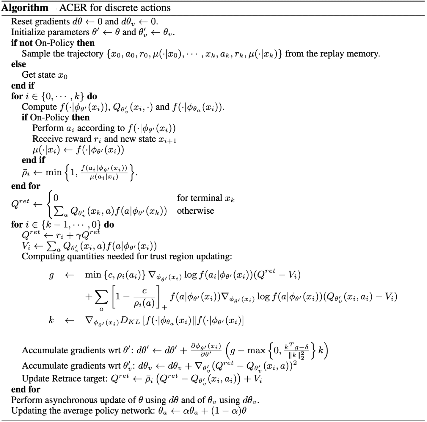
Discrete ACER

Actor Gradient

Off-policy learning with experience replay may seem like a straightforward strategy to enhance the sample efficiency of actor-critics. However, managing the variance and stability of off-policy estimators poses a considerable challenge. Importance sampling stands out as one of the most widely adopted approaches. With the following objective of off-policy actor-critic objective:

\[J (\theta) = \sum_{\mathbf{s} \in \mathcal{S}} \beta (\mathbf{s}) V^{\pi_{\theta}} (\mathbf{s}) = \sum_{\mathbf{s} \in \mathcal{S}} \beta (\mathbf{s}) \sum_{\mathbf{a} \in \mathcal{A}} \pi_{\theta} (\mathbf{a} \vert \mathbf{s}) Q^{\pi_{\theta}} (\mathbf{s}, \mathbf{a}) = \mathbb{E}_{\mathbf{s} \sim \beta, \mathbf{a} \sim \pi_{\theta} (\cdot \vert \mathbf{s})} \left[ Q^{\pi_{\theta}} (\mathbf{s}, \mathbf{a}) \right]\]

where $\beta$ denotes the stationary distribution of behavior policy $\mu$ defined by

\[\beta(\mathbf{s}) = \lim_{t \to \infty} \mathbb{P} (\mathbf{s}_t = \mathbf{s} \vert \mathbf{s}_0, \mu)\]

which $\mathbb{P} (\mathbf{s}_t = \mathbf{s} \vert \mathbf{s}_0, \mu)$ indicates the probability that $\mathbf{s}_t = \mathbf{s}$ when starting in $\mathbf{s}_0$ and executing policy $\mu$. This yields the following approximation of the gradient:

\[\nabla_{\theta} J(\theta) \approx \mathbb{E}_{\mathbf{s}_t \sim \beta_t, \mathbf{a}_t \sim \mu} \left[ \rho_t \nabla_{\theta} \log \pi_\theta (\mathbf{a}_t \vert \mathbf{s}_t) Q^\pi (\mathbf{s}_t, \mathbf{a}_t) \right]\]

where $\rho_t = \pi (\mathbf{a}_t \vert \mathbf{s}_t) / \mu (\mathbf{a}_t \vert \mathbf{s}_t)$ denotes the importance weight.

However, the importance weight usually suffer from vanishing/exploding gradient due to high variance stem from unbounded importance weights $\rho_t = \pi (\mathbf{a}_t \vert \mathbf{s}_t) / \mu (\mathbf{a}_t \vert \mathbf{s}_t)$ are multiplied over timesteps. ACER first truncate the importance weights (ensuring bounded variance) and introduce the bias correction term (ensuring unbiased estimator) via the following decomposition:

\[\begin{aligned} \nabla_{\theta} J(\theta) = & \; \mathbb{E}_{\mathbf{s}_t \sim \beta_t, \color{blue}{\mathbf{a}_t \sim \mu}} \left[ \bar{\rho}_t \nabla_{\theta} \log \pi_\theta (\mathbf{a}_t \vert \mathbf{s}_t) Q^\pi (\mathbf{s}_t, \mathbf{a}_t) \right] \\ & + \mathbb{E}_{\mathbf{s}_t \sim \beta_t, \color{red}{\mathbf{a} \sim \pi}} \left[ \max \left(\frac{\pi (\mathbf{a} \vert \mathbf{s}_t) - c \cdot \mu (\mathbf{a} \vert \mathbf{s}_t)}{\pi (\mathbf{a} \vert \mathbf{s}_t)}, 0 \right) \nabla_{\theta} \log \pi_\theta (\mathbf{a} \vert \mathbf{s}_t) Q^\pi (\mathbf{s}_t, \mathbf{a}) \right] \end{aligned}\]

Then, by further approximations and modifications:

• one-sample MC approximation with $\mathbf{s}_t \sim \beta_t, \mathbf{a}_t \sim \mu$;
• replacing the first $Q^\pi$ leveraging truncated importance weight with retrace estimator $Q^{\mathrm{ret}}$ and the second $Q^\pi$ that we additionally introduced for bias correction with current estimates of critic $Q_\phi$;
• subtracting baseline $V_\phi (\mathbf{s}_t)$;

we obtain the following policy gradient:

\[\begin{aligned} \nabla_{\theta} J(\theta) = & \; \bar{\rho}_t \nabla_{\theta} \log \pi_\theta (\mathbf{a}_t \vert \mathbf{s}_t) \left[Q^\mathrm{ret} (\mathbf{s}_t, \mathbf{a}_t) - V_\phi (\mathbf{s}_t) \right] \\ & + \mathbb{E}_{\color{red}{\mathbf{a} \sim \pi}} \left[ \max \left(\frac{\pi (\mathbf{a} \vert \mathbf{s}_t) - c \cdot \mu (\mathbf{a} \vert \mathbf{s}_t)}{\pi (\mathbf{a} \vert \mathbf{s}_t)}, 0 \right) \nabla_{\theta} \log \pi_\theta (\mathbf{a} \vert \mathbf{s}_t) \left[ Q_\phi (\mathbf{s}_t, \mathbf{a}) - V_\phi (\mathbf{s}_t) \right] \right] \end{aligned}\]

Furthermore, ACER limit the per-step changes to the policy by novel trust region policy optimization to ensure stability. It decomposes policy network $\pi_\theta (\cdot \vert \mathbf{s}) = f(\cdot \vert \psi_\theta (\mathbf{s}))$ in distribution $f$, and a deep neural network that generates the statistics $\psi_\theta (\mathbf{s})$ of this distribution. And, define the average policy network $\psi_{\theta_a}$ and update its parameters $\theta_a$ softly after each update to the policy parameter $\theta$; $\theta_a \leftarrow \alpha \theta_a + (1 - \alpha) \theta$. Then the ACER policy gradient, but with respect to $\psi$, $\nabla_{\psi} J(\theta)$. Then, trust region update involves two stages:

1. optimization problem with linearized KL constraint
   $$ \begin{aligned} & \underset{\mathbf{z}}{\operatorname{ minimize }} \frac{1}{2} \lVert \nabla_{\psi} J(\theta) - \mathbf{z} \rVert_2^2 \\ & \text { subject to } \nabla_{\psi_\theta\left(\mathbf{s}_t\right)} \mathrm{KL}\left[f\left(\cdot \vert \psi_{\theta_a}\left(\mathbf{s}_t\right)\right) \Vert f\left(\cdot \vert \psi_\theta\left(\mathbf{s}_t\right)\right)\right]^\top \mathbf{z} \leq \delta \end{aligned} $$ which solution has a closed form with quadratic programming: $$ \mathbf{z}^* = \nabla_{\psi} J(\theta) - \max\left\{ 0, \frac{\mathbf{k}^\top \nabla_{\psi} J(\theta) - \delta}{\Vert \mathbf{k} \Vert_2^2} \right\} \cdot \mathbf{k} $$ where $\mathbf{k} = \nabla_{\psi_\theta\left(\mathbf{s}_t\right)} \mathrm{KL}\left[f\left(\cdot \vert \psi_{\theta_a}\left(\mathbf{s}_t\right)\right) \Vert f\left(\cdot \vert \psi_\theta\left(\mathbf{s}_t\right)\right)\right]$. Note that if the constraint is satisfied, there is no change to our policy gradient $\nabla_{\psi} J(\theta)$. Otherwise, the update is scaled down in the direction of $\mathbf{k}$, lowering rate of change between the activations of the current policy and the average policy network.
2. Back-propagation
   The updated gradient with respect to $\psi$, $\mathbf{z}^*$, is back-propagated through the network. The parameter updates for the policy network follow from the chain rule $\frac{\partial \psi_{\theta} (\mathbf{s})}{\partial \theta} \mathbf{z}^*$.

Critic Gradient

To estimate $Q^\pi$, ACER employs Retrace algorithm with $\lambda = 1$ as a target. Consider the following identity from the Bellman equation and importance sampling for constructing Q-target:

\[Q^\pi (\mathbf{s}_t, \mathbf{a}_t) = r (\mathbf{s}_t, \mathbf{a}_t) + \gamma \mathbb{E}_{\mathbf{s} \sim \beta, \mathbf{a} \sim \mu} [\rho_{t+1} Q^\pi (\mathbf{s}_{t+1}, \mathbf{a}_{t+1}) ]\]

By using the truncation and bias correction trick, we can derive the formula:

\[\begin{aligned} Q^\pi (\mathbf{s}_t, \mathbf{a}_t) = & \; r (\mathbf{s}_t, \mathbf{a}_t) + \gamma \mathbb{E}_{\mathbf{s} \sim \beta, \color{blue}{\mathbf{a} \sim \mu}} \left[ \bar{\rho}_{t+1} Q^\pi (\mathbf{s}_{t+1}, \mathbf{a}_{t+1}) \right] \\ & + \gamma \mathbb{E}_{\mathbf{s} \sim \beta, \color{red}{\mathbf{a} \sim \pi}} \left[ \max \left(\frac{\pi (\mathbf{a} \vert \mathbf{s}_{t+1}) - c \cdot \mu (\mathbf{a} \vert \mathbf{s}_{t+1})}{\pi (\mathbf{a} \vert \mathbf{s}_{t+1})}, 0 \right) Q^\pi (\mathbf{s}_{t+1}, \mathbf{a}_{t+1}) \right] \end{aligned}\]

Note that this equation is equivalent to Retrace estimator $Q^{\mathrm{ret}}$; by recursively expanding $Q^\pi$, we can represent $Q^\pi (\mathbf{s}, \mathbf{a})$ as

\[Q^\pi(\mathbf{s}, \mathbf{a}) = \mathbb{E}_{\mu} \left[\sum_{t \geq 0} \gamma^t\left(\prod_{t^{\prime}=1}^t \bar{\rho}_{t^\prime} \right)\left(r (\mathbf{s}_t, \mathbf{a}_t) + \gamma \mathbb{E}_{\mathbf{b} \sim \pi} \left[\max \left(\frac{\pi (\mathbf{a} \vert \mathbf{s}_{t+1}) - c \cdot \mu (\mathbf{a} \vert \mathbf{s}_{t+1})}{\pi (\mathbf{a} \vert \mathbf{s}_{t+1})}, 0 \right) Q^\pi\left(\mathbf{s}_{t+1}, \mathbf{b}\right)\right)\right]\right]\]

where $\mathbb{E}_{\mu}$ is taken over trajectories starting from $\mathbf{s}$ with actions generated with respect to $\mu$. Hence, we rewrite $Q^\pi$ in the first equation by $Q^{\mathrm{ret}}$. Subsequently, by taking one-sample MC approximation $\mathbf{s} \sim \beta$ and $\mathbf{a} \sim \mu$, replacing the first $Q^\pi$ leveraging truncated importance weight with $Q^{\mathrm{ret}}$ and the second $Q^\pi$ that we additionally introduced for bias correction with current estimates of critic:

\[Q^{\mathrm{ret}} (\mathbf{s}_t, \mathbf{a}_t) = r (\mathbf{s}_t, \mathbf{a}_t) + \gamma \bar{\rho}_{t+1} Q^{\mathrm{ret}} (\mathbf{s}_{t+1}, \mathbf{a}_{t+1}) + \gamma \mathbb{E}_{\mathbf{a} \sim \pi} \left[ \max \left(\frac{\pi (\mathbf{a} \vert \mathbf{s}_{t+1}) - c \cdot \mu (\mathbf{a} \vert \mathbf{s}_{t+1})}{\pi (\mathbf{a} \vert \mathbf{s}_{t+1})}, 0 \right) Q_\phi (\mathbf{s}_{t+1}, \mathbf{a}_{t+1}) \right]\]

Again, through the truncation and bias correction trick again for \(V_\phi (\mathbf{s}_t) = \mathbb{E}_{\mathbf{a} \sim \pi}[Q_\phi(\mathbf{s}_t, \mathbf{a})]\) and one-sample MC $\mathbf{a} \sim \mu$ of the first expectation:

\[V_\phi (\mathbf{s}_{t+1}) = \mathbb{E}_{\mathbf{a} \sim \pi}[Q_\phi(\mathbf{s}_t, \mathbf{a})] \approx \bar{\rho}_{t+1} Q_\phi (\mathbf{s}_{t+1}, \mathbf{a}_{t+1}) + \mathbb{E}_{\mathbf{a} \sim \pi} \left[ \max \left(\frac{\pi (\mathbf{a} \vert \mathbf{s}_{t+1}) - c \cdot \mu (\mathbf{a} \vert \mathbf{s}_{t+1})}{\pi (\mathbf{a} \vert \mathbf{s}_{t+1})}, 0 \right) Q_\phi (\mathbf{s}_{t+1}, \mathbf{a}_{t+1}) \right]\]

Finally, we obtain the following target by multiplying the above identity by $\gamma$ and subtracting identity of \(Q^{\mathrm{ret}}\):

\[Q^{\mathrm{ret}} (\mathbf{s}_t, \mathbf{a}_t) = r (\mathbf{s}_t, \mathbf{a}_t) + \gamma \bar{\rho}_{t+1} [Q^{\mathrm{ret}} (\mathbf{s}_{t+1}, \mathbf{a}_{t+1}) - Q_\phi(\mathbf{s}_{t+1}, \mathbf{a}_{t+1}) ] + \gamma V_\phi(\mathbf{s}_{t+1})\]

where \(V_\phi( \mathbf{s} ) = \mathbb{E}_{\mathbf{a} \sim \pi} [Q_\phi(\mathbf{s}, \mathbf{a})]\).

To learn the critic $Q_\phi$, ACER utilizes MSE loss:

\[\mathcal{L}_{\textrm{critic}} (\phi) = \frac{1}{2} \lVert Q_{\phi} (\mathbf{s}_t, \mathbf{a}_t) - Q^{\mathrm{ret}} (\mathbf{s}_t, \mathbf{a}_t) \rVert^2\]

and update $\phi$ with the following standard gradient for each state-action pair:

\[\left[ Q_\phi (\mathbf{s}_t, \mathbf{a}_t) - Q^{\mathrm{ret}} (\mathbf{s}_t, \mathbf{a}_t) \right] \nabla_{\phi} Q_\phi (\mathbf{s}_t, \mathbf{a}_t)\]

$\mathbf{Fig\ 1.}$ Pseudocode for Discrete ACER. (source: Wang et al. 2017)

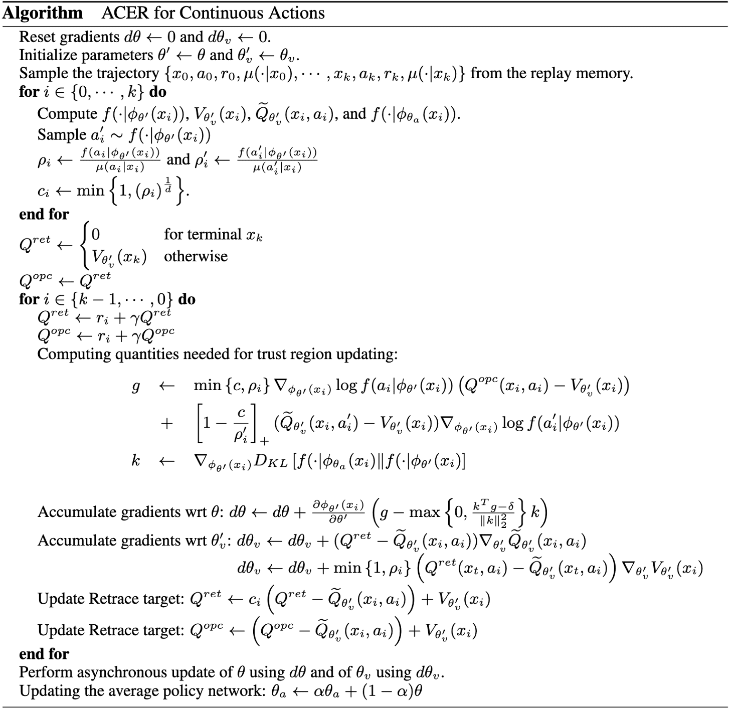
Continuous ACER

Actor Gradient

The overall framework of actor update in continuous action space ACER is equal to discrete case. For the distribution $f$, Gaussian distributions with fixed diagonal covariance and mean $\psi_\theta (\mathbf{s})$ is selected. Moreover, for Q-target, $Q^\pi (\lambda)$ estimator $Q^{\mathrm{opc}}$ is leveraged instead of Retrace estimator $Q^{\mathrm{ret}}$. Recall that it is the same as Retrace with the exception that the truncated importance ratio $\bar{\rho}_t$ is replaced with $1$.

Critic Gradient

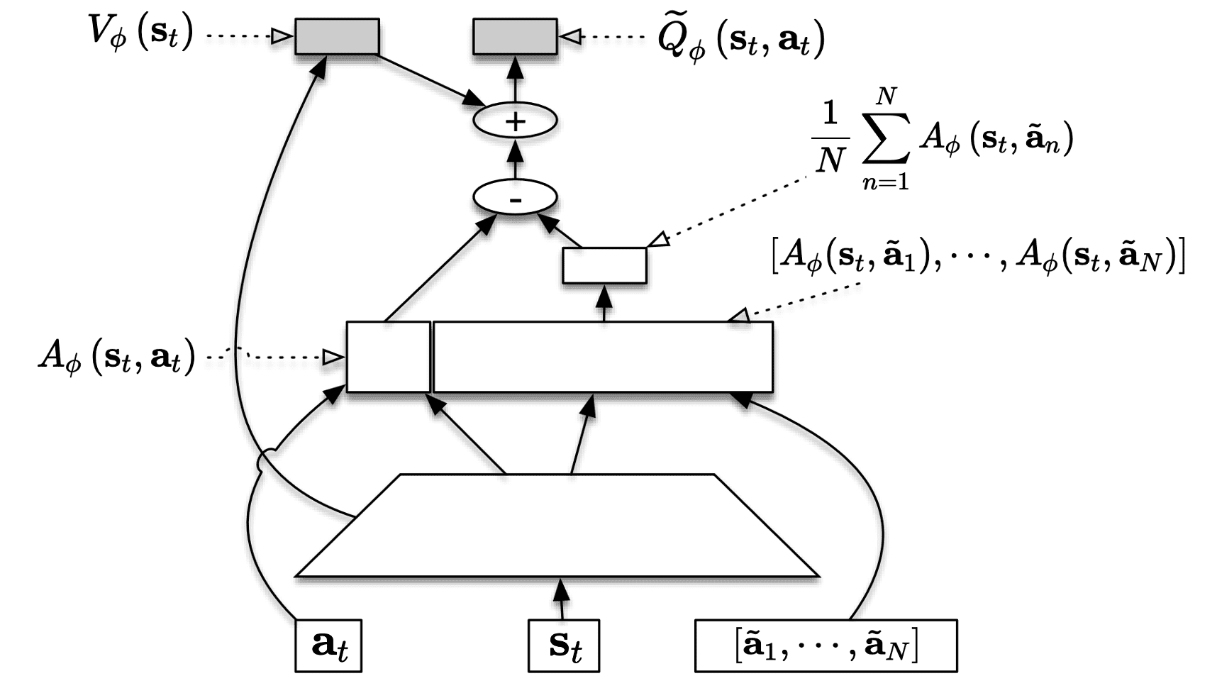
In continuous action spaces, $V$ cannot be easily derived by integrating over $Q$. The authors proposed the extension of dueling network in Dueling DQN that predicts advantage function $A_\phi$, called stochastic dueling networks (SDNs) to estimate both $V^\pi$ and $Q^\pi$ off-policy. At each time step, it outputs a stochastic estimate \(\widetilde{Q}_\phi\) of $Q^\pi$ and a deterministic estimate $V_\phi$ of $V^\pi$:

\[\widetilde{Q}_{\phi} \left(\mathbf{s}_t, \mathbf{a}_t \right) \sim V_{\phi} \left(\mathbf{s}_t\right)+ A_{\phi} \left(\mathbf{s}_t, \mathbf{a}_t \right)-\frac{1}{N} \sum_{n=1}^N A_{\phi} \left(\mathbf{s}_t, \widetilde{\mathbf{a}}_n\right) \text{ where } \widetilde{\mathbf{a}}_n \sim \pi_\theta\left(\cdot \mid \mathbf{s}_t\right)\]

which ensures the consistency in the sense that \(\mathbb{E}_{\mathbf{a} \sim \pi} [\mathbb{E}_{\widetilde{\mathbf{a}}_{1:n} \sim \pi} [\widetilde{Q}_{\phi} \left(\mathbf{s}_t, \mathbf{a}_t \right)]] = V_{\phi} \left(\mathbf{s}_t\right)\).

$\mathbf{Fig\ 2.}$ A schematic of the Stochastic Dueling Network (SDN). (source: Wang et al. 2017)

To obtain target for estimating $V^\pi$, we use similar technique that we utilized to derive a recursive identity of $Q^{\mathrm{ret}}$. Consequently, $V^{\mathrm{target}}$ is given by

\[V^{\mathrm{target}} (\mathbf{s}_t) = \bar{\rho}_t Q^{\mathrm{ret}} (\mathbf{s}_t, \mathbf{a}_t) + \mathbb{E}_{\mathbf{a} \sim \pi} \left[ \max \left(\frac{\pi (\mathbf{a} \vert \mathbf{s}_t) - c \cdot \mu (\mathbf{a} \vert \mathbf{s}_t)}{\pi (\mathbf{a} \vert \mathbf{s}_t)}, 0 \right) Q_\phi (\mathbf{s}_t, \mathbf{a})\right]\]

Through the truncation and bias correction trick again for \(V_\phi (\mathbf{s}_t) = \mathbb{E}_{\mathbf{a} \sim \pi} [Q_\phi (\mathbf{s}_t, \mathbf{a})]\) and one-sample MC \(V_\phi (\mathbf{s}_t) \approx Q_\phi (\mathbf{s}_t, \mathbf{a}_t)\), we obtain the following target by subtracting these identities:

\[V^{\mathrm{target}} (\mathbf{s}_t) = \bar{\rho}_t \left[ Q^\mathrm{ret} (\mathbf{s}_t, \mathbf{a}) - Q_\phi (\mathbf{s}_t, \mathbf{a}_t) \right] + V_\phi (\mathbf{s}_t)\]

As a minor detail, which is not essential but leads to the fast convergence of training, the truncated importance weights in $Q^{\mathrm{ret}}$ is modified as $\min (1, \rho_t^{1/d})$ where $d$ is the dimensionality of the action space $\mathcal{A}$.

$\mathbf{Fig\ 3.}$ Pseudocode for Continuous ACER. (source: Wang et al. 2017)

Deep Deterministic Policy Gradient (DDPG)

The DQN algorithm has demonstrated its efficacy in addressing challenges associated with observation spaces of high dimensionality such as Atari games; however, it is constrained to handling discrete and low-dimensional action spaces. This limitation stems from the inability of DQN to seamlessly operate within continuous domains, as it relies on the $\arg \max$ operation of the action-value function, necessitating an iterative optimization process at each step in cases of continuous valued domains.

In response to this constraint, Lillicrap et al. 2016 proposed an off-policy actor-critic approach, which integrates DQN with the deterministic policy gradient (DPG), called Deep Deterministic Policy Gradient (DDPG). Instead of intensive optimizations to determine $\max_\mathbf{a} Q_\phi (\mathbf{s}, \mathbf{a})$, DDPG expands the scope of DQN critic to encompass continuous action space by learning deterministic actor $\mu_\theta$ to approximate $\max_\mathbf{a} Q_\phi (\mathbf{s}, \mathbf{a}) \approx Q_\phi (\mathbf{s}, \mu_\theta (\mathbf{a}))$.

Deterministic Policy Gradient (DPG)

Recall that the policy gradient theorem is proved by assuming that the policy $\pi_{\theta}$ is stochastic: $\pi_\theta (\mathbf{a} \vert \mathbf{s}) = \mathbb{P}[\mathbf{a} \vert \mathbf{s}; \theta]$

\[\nabla_\theta V(\theta) = \mathbb{E}_{\tau \sim p_\theta} [ \nabla_\theta \text{ log } \pi_\theta (\mathbf{a} \vert \mathbf{s}) Q_{\pi_\theta} (\mathbf{s}, \mathbf{a})]\]

However, it is not specified that deterministic policy $\mathbf{a} = \mu_{\theta} (\mathbf{s})$ also satisfies the theorem. Then the natural question arises here:

Can we have deterministic policy gradient? Does the policy gradient theorem also hold for deterministic policies?

Silver et al. PMLR 2014 proved that the deterministic policy gradient does indeed exist, and furthermore it has a simple model-free form that simply follows the gradient of the action-value function.

Consider a deterministic policy $\mu_\theta: \mathcal{S} \to \mathcal{A}$ with parameter vector $\theta \in \mathbb{R}^n$, and we define an objective function analogously to the stochastic case as follows:

\[J(\theta) = \int_{\mathcal{S}} \rho^\mu (\mathbf{s}) Q(\mathbf{s}, \mu_\theta (\mathbf{s})) \; d \mathbf{s} = \mathbb{E}_{\mathbf{s} \sim \rho^\mu} [Q(\mathbf{s}, \mathbf{a} = \mu_{\theta} (\mathbf{s}))]\]

where

• $\rho_0 (\mathbf{s})$: the initial distribution over states;
• $\rho^\mu (\mathbf{s} \to \mathbf{s}^\prime, k)$: starting from state $\mathbf{s}$, the visitation probability density at state $\mathbf{s}^\prime$ after moving $k$ steps by policy $\mu$;
• $\rho^\mu (\mathbf{s}^\prime)$: discounted state distribution, defined as

\[\rho^\mu\left(\mathbf{s}^{\prime}\right)=\int_{\mathcal{S}} \sum_{k=1}^{\infty} \gamma^{k-1} \rho_0(\mathbf{s}) \rho^\mu\left(\mathbf{s} \rightarrow \mathbf{s}^{\prime}, k\right) d \mathbf{s}\]

And according to the Leibniz integral rule to exchange derivative and integral and the chain rule, we can first take the gradient of $Q$ with regard to the action $\mathbf{a}$ and then take the gradient of the deterministic policy function $\mu$ with regard to $\theta$ (the rigorous proof is provided in the below statement):

$\color{red}{\mathbf{Thm.}}$ Deterministic Policy Gradient Theorem
For any differentiable deterministic policy $\mathbf{a} = \mu_\theta ( \mathbf{s} )$ with some regularity conditions:

1. The following quantities are continuous in its all parameters and variables: $$ \mathbb{P}(\mathbf{s}^\prime \vert \mathbf{s}, \mathbf{a}), \; \nabla_{\mathbf{a}} \mathbb{P}(\mathbf{s}^\prime \vert \mathbf{s}, \mathbf{a}), \; \mu_{\theta} (\mathbf{s}), \; \nabla_{\theta} \mu_{\theta} (\mathbf{s}), \; r(\mathbf{s}, \mathbf{a}), \; \nabla_{\mathbf{a}} (\mathbf{s}, \mathbf{a}), \; \rho_0 (\mathbf{s}) $$
2. There exists constants $b$ such that $$ \sup_{\mathbf{s}} \rho_0 (\mathbf{s}), \; \sup_{\mathbf{a}, \mathbf{s}, \mathbf{s}^\prime} \mathbb{P}(\mathbf{s}^\prime \vert \mathbf{s}, \mathbf{a}), \; \sup_{\mathbf{a}, \mathbf{s}} r(\mathbf{s}, \mathbf{a}) < b $$ and $L$ such that $$ \sup_{\mathbf{a}, \mathbf{s}, \mathbf{s}^\prime} \lVert \nabla_{\mathbf{a}} \mathbb{P}(\mathbf{s}^\prime \vert \mathbf{s}, \mathbf{a}) \rVert, \; \sup_{\mathbf{a}, \mathbf{s}} \lVert \nabla_{\mathbf{a}} r(\mathbf{s}, \mathbf{a}) \rVert < L. $$

the deterministic policy gradient is then given by $$ \begin{aligned} \nabla_\theta J(\theta) & =\int_{\mathcal{S}} \left.\rho^\mu(\mathbf{s}) \nabla_{\mathbf{a}} Q^\mu(\mathbf{s}, \mathbf{a}) \nabla_\theta \mu_\theta(\mathbf{s})\right|_{\mathbf{a}=\mu_\theta(\mathbf{s})} d \mathbf{s} \\ & =\mathbb{E}_{\mathbf{s} \sim \rho^\mu}\left[\left.\nabla_{\mathbf{a}} Q^\mu(\mathbf{s}, \mathbf{a}) \nabla_\theta \mu_\theta(\mathbf{s})\right|_{\mathbf{a}=\mu_\theta(\mathbf{s})}\right] \end{aligned} $$

$\mathbf{Proof.}$

The proof follows a similar scheme to the stochastic policy gradient theorem that I proved in the past post. The proof might be tedious but can be simply done with the definition, Leibniz integral rule, and Fubini theorem, which are valid by assuming the regularity conditions. For more detail, see the supplementary.

\[\tag*{$\blacksquare$}\]

Thus, the deterministic policy can be more efficient to learn because its gradient only requires to integrate the stochasticity in state visitation, while the stochastic policy gradient should consider the randomness in both state visitation and action. However, it is important to observe the following pros and cons between deterministic and stochastic policies:

	Deterministic	Stochastic
Pros	efficient to learn	naturally encourages exploration due to randomness
Cons	limited exploration due to the absence of stochasticity	its variance becomes basically larger and need to get more samples to get a gradient

This observation implies that behaving according to a deterministic policy can be disastrous in certain scenarios. For instance, in environments with minimal stochasticity, using a deterministic policy may not yield effective results, or it may be exceedingly challenging to achieve success.

In such cases, the deterministic policy gradient can be modified into off-policy via the same technique that we utilized in stochastic case, with arbitary behavior policy $\beta(\mathbf{a} \vert \mathbf{s})$:

\[\begin{aligned} \nabla_\theta J_\beta\left(\mu_\theta\right) & \approx \int_{\mathcal{S}} \rho^\beta(\mathbf{s}) \nabla_\theta \mu_\theta(a \mid s) Q^\mu(\mathbf{s}, \mathbf{a}) \mathrm{d} \mathbf{s} \\ & =\mathbb{E}_{\mathbf{s} \sim \rho^\beta}\left[\left.\nabla_\theta \mu_\theta(\mathbf{s}) \nabla_{\mathbf{a}} Q^\mu(\mathbf{s}, \mathbf{a})\right|_{\mathbf{a}=\mu_\theta(\mathbf{s})}\right] \end{aligned}\]

From DQN to DDPG: Deep Q-Learning for continuous action spaces

In the context of exploration, Q-Learning may seem appealing as it is an off-policy algorithm that does not require importance weights, which can increase the variance. However, applying Q-Learning to continuous action spaces poses challenges, particularly because action selection and $Q$-target calculations rely on the $\textrm{argmax}$ and $\max$ operator. While feasible for finite action spaces $\mathcal{A}$, continuous action spaces present difficulties in this regard.

\[\pi (\mathbf{s}) = \underset{\mathbf{a} \in \mathcal{A}}{\textrm{ arg max }} Q^* (\mathbf{s}, \mathbf{a}) \\ \widehat{y} = r(\mathbf{s}, \mathbf{a}) + \gamma \underset{\mathbf{a}^\prime \in \mathcal{A}}{\max} Q(\mathbf{s}^\prime, \mathbf{a}^\prime)\]

Deep Deterministic Policy Gradient (DDPG) introduced in Lillicrap et al. ICLR 2016 extends DQN to continous action spaces with DPG algorithm by presuming that the action is generated from a differentiable deterministic policy $\mu_\theta (\mathbf{s})$, try to approximate

\[\underset{\mathbf{a} \in \mathcal{A}}{\max} Q (\mathbf{s}, \mathbf{a}) = \underset{\theta \in \mathcal{\Theta}}{\max} Q (\mathbf{s}, \mu_{\theta} (\mathbf{s}))\]

DDPG implements this by using a target actor network $\mu_{\theta_{\textrm{targ}}} (\mathbf{s})$ to compute an action which approximately maximizes $Q_{\phi_{\text{targ}}}$, i.e.

\[\underset{\mathbf{a} \in \mathcal{A}}{\max} Q_{\phi_{\text{targ}}} (\mathbf{s}, \mathbf{a}) \approx Q_{\phi_{\text{targ}}} (\mathbf{s}, \mu_{\theta_{\textrm{targ}}} (\mathbf{s}))\]

• DQN
  • Update the Q-Network to minimize the following w.r.t. $\phi$ and periodically update the target network by replacing $\phi_{\textrm{targ}}$ with the $\phi$:
  \[L(\phi) = \mathbb{E}_{(\mathbf{s}, \mathbf{a}, r, \mathbf{s}^\prime) \sim \mathcal{D}} \left[ \left( \color{blue}{r + \gamma \underset{\mathbf{a}^\prime \in \mathcal{A}}{\max} Q_{\phi_{\textrm{targ}}} (\mathbf{s}^\prime, \mathbf{a}^\prime)} - \color{red}{Q_{\phi} (\mathbf{s}, \mathbf{a})} \right)^2 \right]\] \[\begin{aligned} \phi & \leftarrow \phi + \eta_t \nabla_{\phi} L (\phi) \\ \phi_{\textrm{targ}} & \leftarrow \phi \end{aligned}\]
• DDPG

  • Update Critic to minimize the following w.r.t. $\phi$ (same as DQN) and periodical soft target update with $\rho \approx 1$ to improve the stability of learning:

    \[L(\phi) = \mathbb{E}_{(\mathbf{s}, \mathbf{a}, r, \mathbf{s}^\prime) \sim \mathcal{D}} \left[ \left( \color{blue}{r + \gamma Q_{\phi_{\textrm{targ}}} (\mathbf{s}^\prime, \mu_{\theta_{\textrm{targ}}} (\mathbf{s}^\prime))} - \color{red}{Q_{\phi} (\mathbf{s}, \mathbf{a})} \right)^2 \right]\] \[\begin{aligned} \phi_{\textrm{targ}} & \leftarrow \rho \phi_{\textrm{targ}} + (1 - \rho) \phi \\ \theta_{\textrm{targ}} & \leftarrow \rho \theta_{\textrm{targ}} + (1 - \rho) \theta \\ \end{aligned}\]

  • Update Actor by using deterministic policy gradient:

    \[\nabla_{\theta} J(\theta) = \mathbb{E}_{(\mathbf{s}, \mathbf{a}, r, \mathbf{s}^\prime) \sim \mathcal{D}} \left[ \nabla_{\mathbf{a}} Q_{\phi} (\mathbf{s}, \mathbf{a} = \mu_{\theta} (\mathbf{s})) \nabla_{\theta} \mu_{\theta} (\mathbf{s}) \right]\]

The entire algorithm is outlined in the pseudocode below:

$\mathbf{Fig\ 1.}$ The pseudocode for DDPG algorithm (OpenAI)

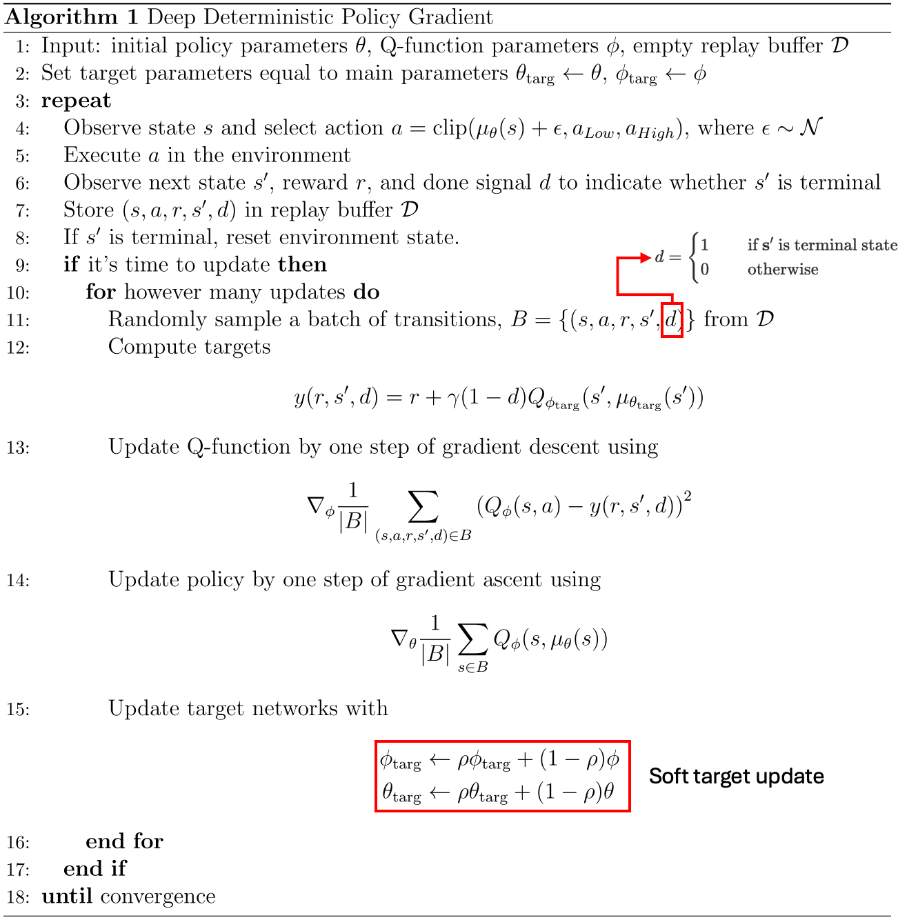
It is worthwhile to note some details regarding exploration. Since the DDPG policy is deterministic, it might not explore a wide enough range of actions to discover valuable learning signals. To enhance the exploration, additional noise is incorporated into the actions as one can see in the pseudocode. While the original DDPG paper suggested using time-correlated Ornstein-Uhlenbeck noise, recent findings indicate that simple mean-zero Gaussian noise is equally effective and is therefore preferred.

Twin-Delayed DDPG (TD3)

The Q-learning algorithm is known to suffer from the overestimation of the value function. This challenge persists in an actor-critic setting, especially with deterministic actor, and is thus possible to adversely impact the policy. Twin-Delayed Deep Deterministic policy gradient (TD3), proposed by Fujimoto et al., 2018 implemented several techniques on top of DDPG (i.e. deterministic $\pi_\theta$) to mitigate the overestimation of the value function.

$\mathbf{Fig\ 4.}$ Overestimation Bias in the value estimates of DDPG.
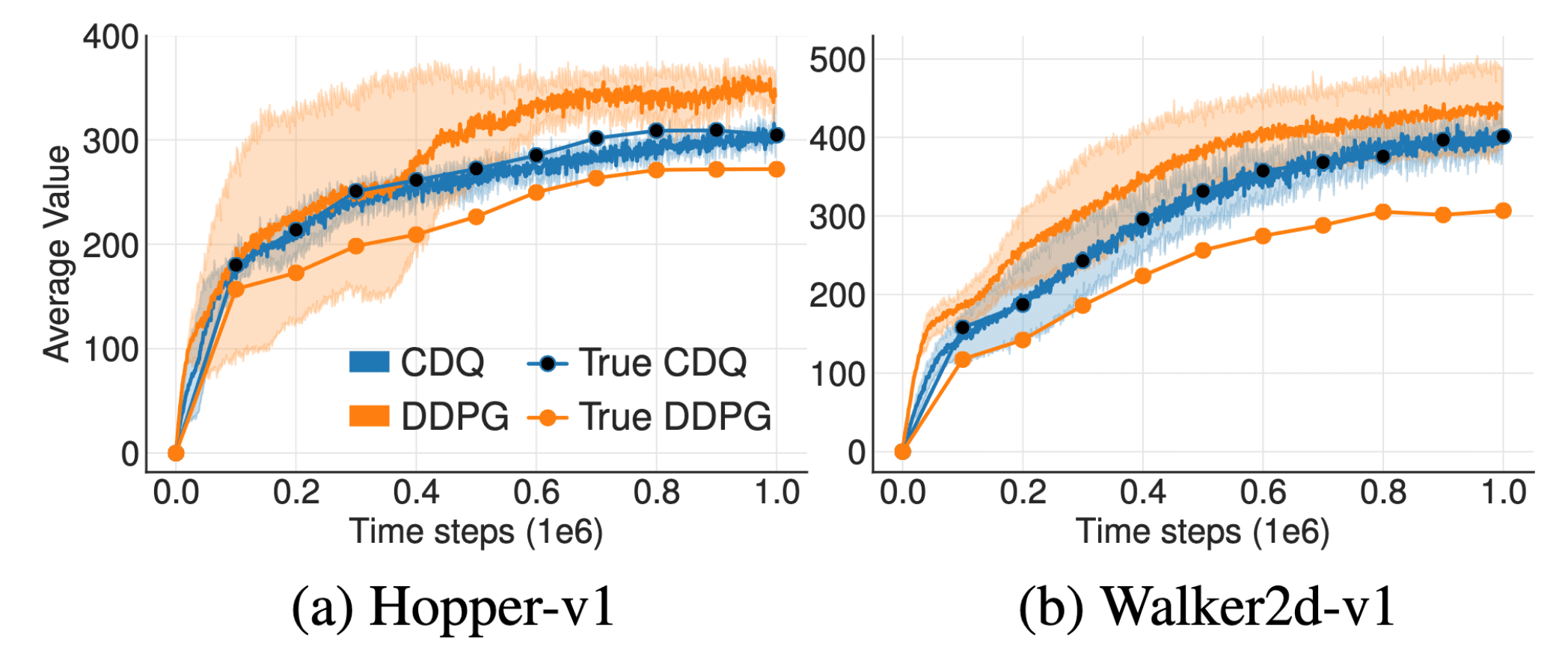
Proposed Clipped Double Q-learning (CDQ) of TD3 can effectively reduce such bias. (source: Fujimoto et al. 2018)

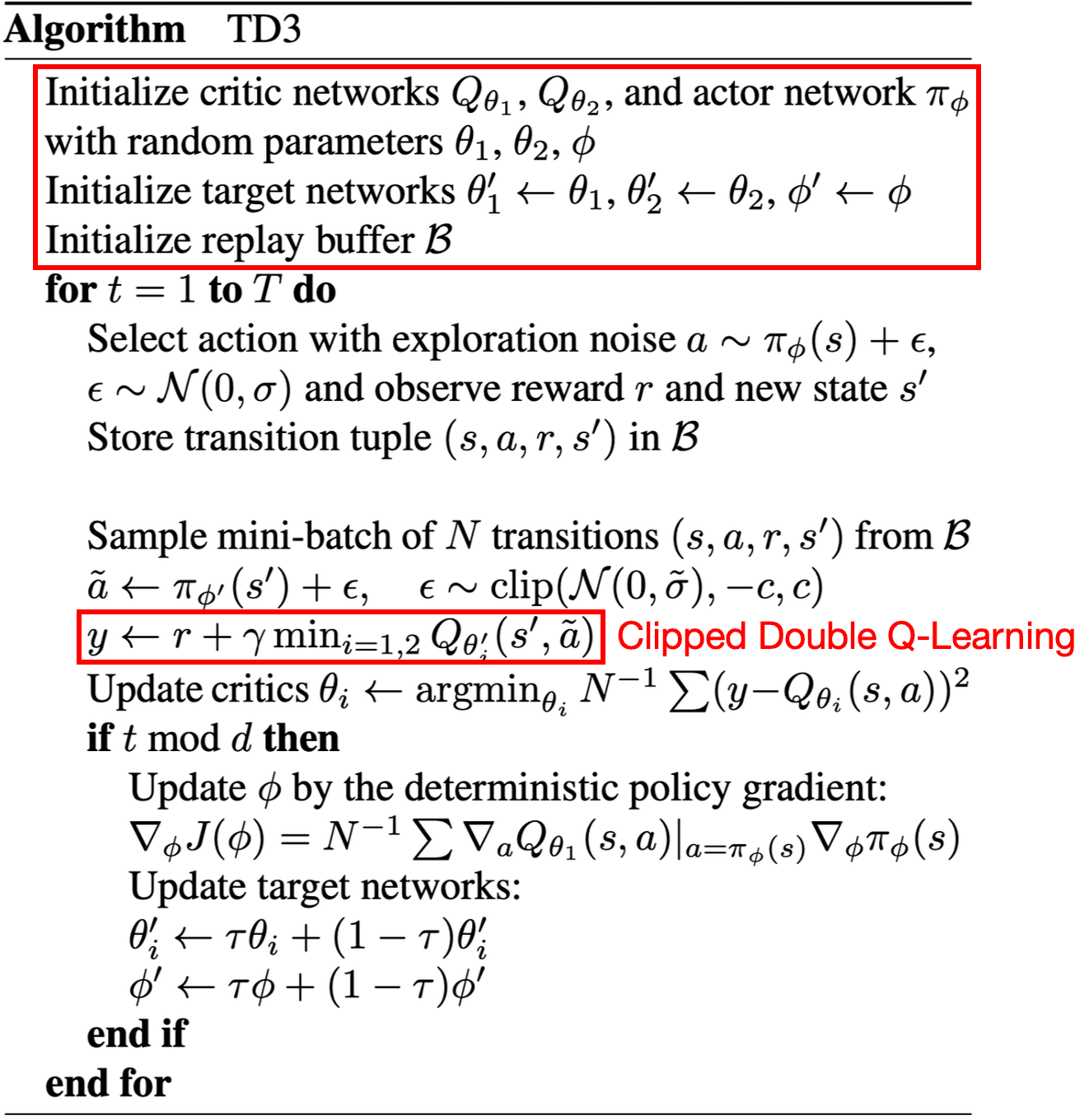
Clipped Double Q-Learning

Recall that the $\max$ operator in standard Q-learning uses the identical values both for action selection and evaluation, thus increasing the likelihood of selecting overestimated values and yielding overly optimistic value estimates. And also recall that double Q-Learning learns two different Q-values $Q_{\phi_1}$ and $Q_{\phi_2}$ by assigning each experience randomly to update one of the two Q-value functions. Consequently, the agent can disentangles the selection and evaluation processes in Q-learning and revises its target as follows:

\[r (\mathbf{s}, \mathbf{a}) + \gamma \cdot Q (\mathbf{s}^\prime, \pi_{\phi} (\mathbf{s}^\prime); \phi^\prime) \text{ where } \pi_{\phi} (\mathbf{s}^\prime) = \underset{\mathbf{a}^\prime \in \mathcal{A}}{\arg\max} \; Q (\mathbf{s}^\prime, \mathbf{a}^\prime; \phi)\]

where $\phi$ and $\phi^\prime$ are randomly selected among $\phi_1$ and $\phi_2$. In actor-critic setting, this formulation is equivalent to the following Q target of a pair of critics $(Q_{\phi_1}, Q_{\phi_2})$ of which actors $(\pi_{\theta_1}, \pi_{\theta_2})$, with target actors $(\pi_{\theta_1^\prime}, \pi_{\theta_2^\prime})$ and target critics $(Q_{\phi_1^\prime}, Q_{\phi_2^\prime})$:

\[\begin{aligned} \text{ Q-target of } Q_{\phi_1}: \quad & r (\mathbf{s}, \mathbf{a}) + \gamma Q_{\phi_1^\prime}(\mathbf{s}^\prime, \pi_{\theta_1^\prime}(\mathbf{s}^\prime))\\ \text{ Q-target of } Q_{\phi_2}: \quad & r (\mathbf{s}, \mathbf{a}) + \gamma Q_{\phi_2^\prime}(\mathbf{s}^\prime, \pi_{\theta_2^\prime}(\mathbf{s}^\prime)) \end{aligned}\]

Since two pairs are not entirely independent, due to the use of the opposite critic in the learning targets, as well as the same replay buffer, it is empirically demonstrated that it does not entirely eliminate the overestimation. Instead, clipped double Q-learning is simply implemented to be underestimated rather than overestimated:

\[\begin{aligned} & r (\mathbf{s}, \mathbf{a}) + \gamma \underset{n = 1, 2}{\min} Q_{\phi_n^\prime}(\mathbf{s}^\prime, \pi_{\theta_1^\prime}(\mathbf{s}^\prime))\\ & r (\mathbf{s}, \mathbf{a}) + \gamma \underset{n = 1, 2}{\min} Q_{\phi_n^\prime}(\mathbf{s}^\prime, \pi_{\theta_2^\prime}(\mathbf{s}^\prime)) \end{aligned}\]

While this update rule induces an underestimation bias, this is less likely to be propagated as underestimated actions will not be explicitly reinforced through the policy update. Additionally, in TD3, these update rules can be approximated with single actor $\pi_\theta$ optimized with respect to $Q_\phi$ for the sake of efficiency. If $Q_{\phi_1} > Q_{\phi_2}$, Q-target for both critics remains identical; otherwise, the Q-target is reduced similar to Double Q-learning framework.

$\mathbf{Fig\ 5.}$ Pseudocode for TD3: Clipped Double Q-Learning. (source: Fujimoto et al. 2018)

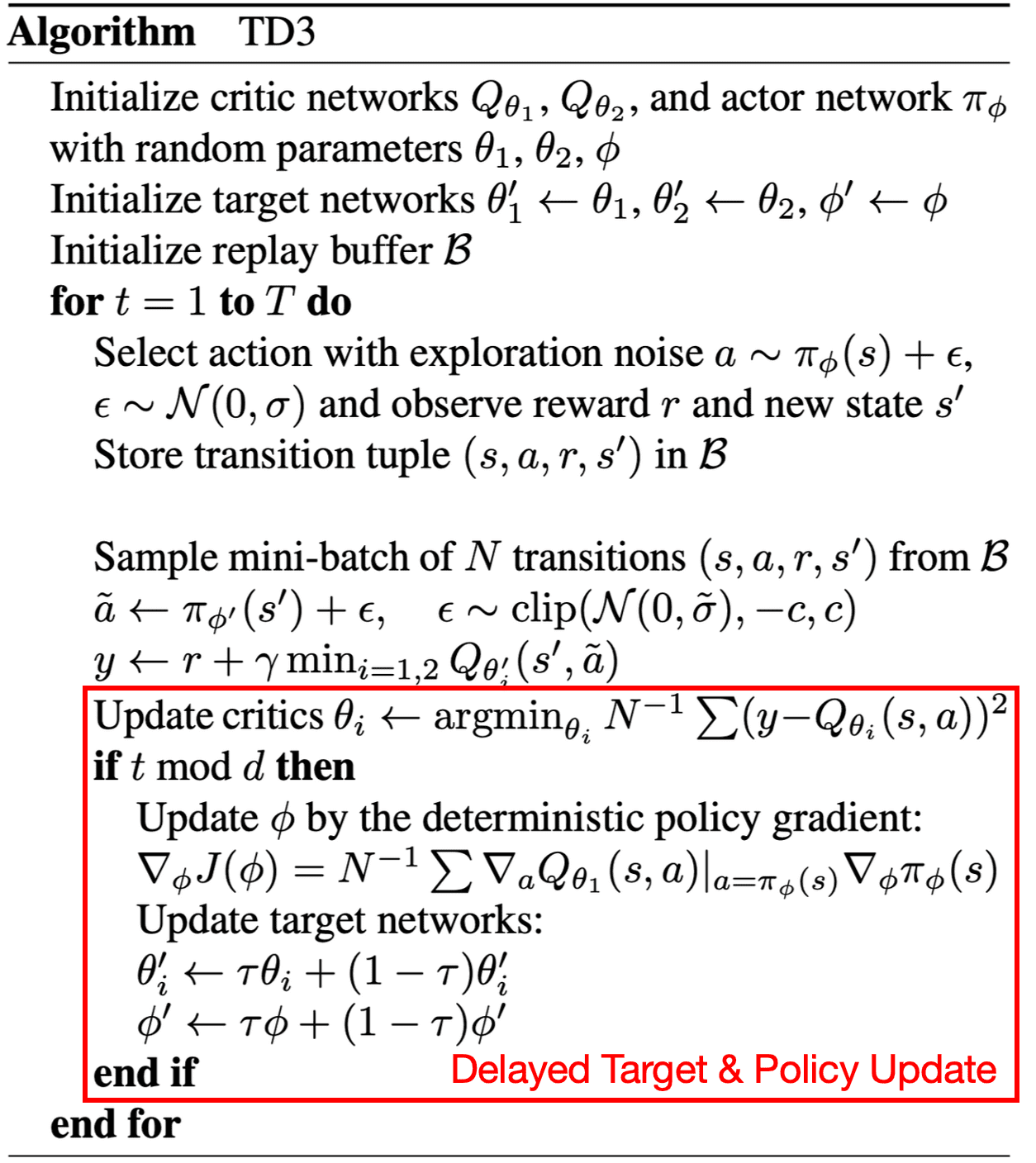
Delayed Target & Policy Updates

The authors observed that actor-critic methods can fail to learn due to the interplay between the actor and critic updates. Value estimates diverge through overestimation when the policy is poor, and the policy will become poor if the value estimate itself is inaccurate.

To avoid such divergent behaviors and further reduce the variance, TD3 proposed to slowly update the policy and target networks of DDPG after a fixed number of updates $d$ to the critic. This is analogous to the slow update of target networks in DQN frameworks.

$\mathbf{Fig\ 6.}$ Pseudocode for TD3: Delayed Target and Policy Updates. (source: Fujimoto et al. 2018)

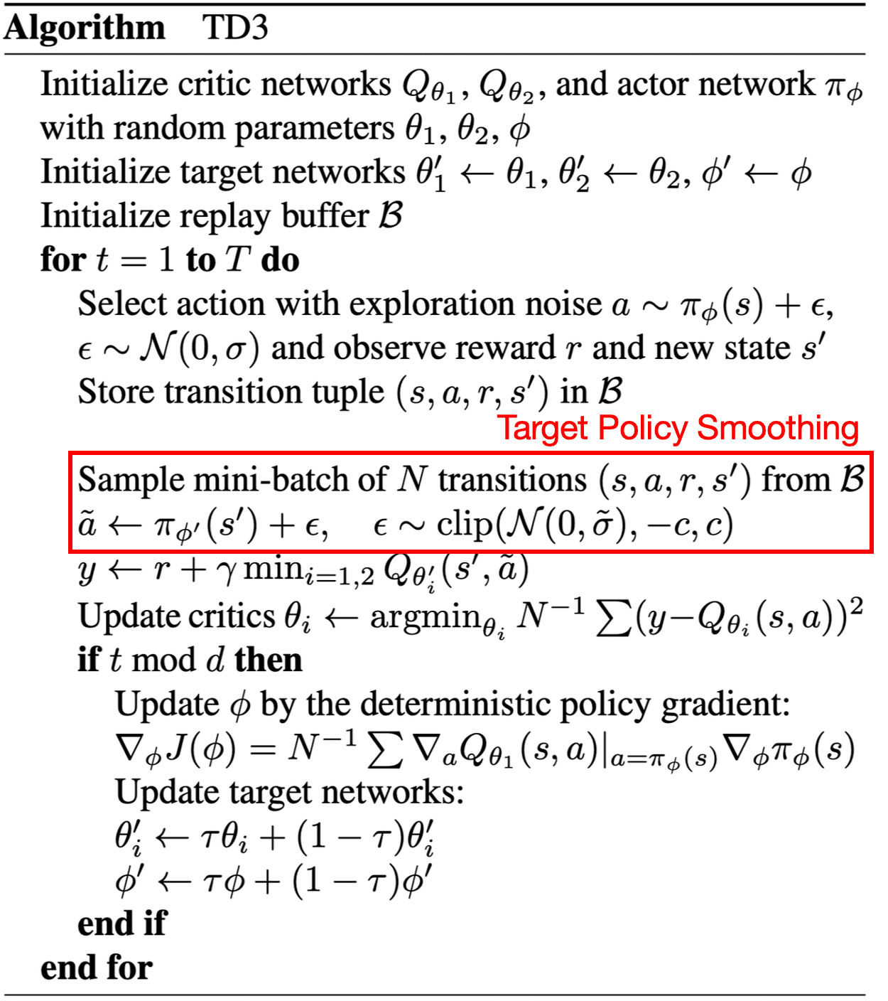
Target Policy Smoothing

When updating the critic, a learning target using a deterministic policy is highly susceptible to inaccuracies induced by function approximation error, increasing the variance of the target. Furthermore, deterministic policies can easily overfit to narrow peaks in the value function.

TD3 introduced a smoothing regularization strategy on the value function: adding a small amount of clipped random noises to the selected action and averaging over mini-batches:

\[\begin{gathered} y = r (\mathbf{s}, \mathbf{a}) + \gamma Q_{\phi^\prime} (\mathbf{s}^\prime, \pi_{\theta^\prime}(\mathbf{s}^\prime) + \epsilon) \\ \text{ where } \epsilon \sim \text{clip}(\mathcal{N}(0, \sigma), -c, +c) \end{gathered}\]

Fitting the value of narrow area around the target action offers the advantage of smoothing the value estimate by leveraging similar state-action value estimates. This approach enforces the idea that similar actions should yield similar values and mimics the expected update rule of expected SARSA:

\[\underbrace{y = r (\mathbf{s}, \mathbf{a}) + \gamma \mathbb{E}_{\mathbf{a}^\prime \sim \mu} \left[ Q (\mathbf{s}^\prime, \mathbf{a}^\prime) \right]}_{\text{Expected SARSA}} \Leftrightarrow \underbrace{y = r (\mathbf{s}, \mathbf{a}) + \gamma \mathbb{E}_{\epsilon} \left[ Q_{\phi^\prime} (\mathbf{s}^\prime, \pi_{\theta^\prime}(\mathbf{s}^\prime) + \epsilon) \right]}_{\text{TD3}}\]

$\mathbf{Fig\ 7.}$ Pseudocode for TD3: Target Policy Smoothing. (source: Fujimoto et al. 2018)

Soft Actor-Critic (SAC)

The combination of off-policy learning and high-dimensional, nonlinear function approximation with neural networks presents a major challenge for stability and convergence. In off-policy actor-critic, a commonly used algorithm DDPG provides for sample-efficient learning on both discrete and continuous action spaces, but t he interplay between the deterministic actor network and the Q-function typically makes DDPG extremely difficult to stabilize and brittle to hyperparameter settings.

Haarnoja et al. 2018 presented Soft Actor Critic (SAC), a sample-efficient and stable off-policy actor-critic algorithm with stochastic policy, forming a bridge between stochastic policy optimization and DDPG-style approaches.

Entropy-Regularized RL

Entropy-regularized RL, a specific technique within the framework of Maximum entropy RL aims to optimize policies to maximize both the expected return and the expected entropy of the policy through the inclusion of an entropy regularization loss. This framework has been used in many contexts, spanning from inverse reinforcement learning to optimal control. Throughout various academic works, the maximum entropy objective has demonstrated its conceptual and practical advantages. By maximizing entropy, the policy is enforced to explore more broadly, and is thus possible to capture mutliple modes of near-optimal behavior.

\[\pi^* = \underset{\pi}{\arg \max} \; \mathbb{E}_{\tau \sim \pi} \left[ \sum_{t=0} \gamma^t \Big( r (\mathbf{s}_t, \mathbf{a}_t) + \alpha \mathbb{H}[\pi (\cdot \vert \mathbf{s}_t)] \Big) \right] \text{ where } \mathbb{H}(\mathbb{P}) = \mathbb{E}_{\mathbf{x} \sim \mathbb{P}} [ - \log \mathbb{P}(\mathbf{x}) ]\]

The temperature parameter $\alpha$ governs the relative importance of the entropy term in contrast to the reward, thereby regulating the stochasticity of the optimal policy. Consequently, this adjusted objective function induces the subsequent alterations in the value functions:

\[\begin{aligned} V^\pi (\mathbf{s}) & = \mathbb{E}_{\tau \sim \pi} \left. \left[ \sum_{t=0} \gamma^t \Big( r (\mathbf{s}_t, \mathbf{a}_t) + \alpha \mathbb{H}[\pi (\cdot \vert \mathbf{s}_t)] \Big) \right\vert \mathbf{s}_0 = \mathbf{s} \right] \\ Q^\pi (\mathbf{s}, \mathbf{a}) & = \mathbb{E}_{\tau \sim \pi} \left. \left[ \sum_{t=0} \gamma^t r (\mathbf{s}_t, \mathbf{a}_t) + \alpha \sum_{t=1} \gamma^t \mathbb{H}[\pi (\cdot \vert \mathbf{s}_t)] \right\vert \mathbf{s}_0 = \mathbf{s}, \mathbf{a}_0 = \mathbf{a} \right] \\ \end{aligned}\]

These modified value functions are called soft value functions. Also, Bellman equations are modified as:

\[\begin{aligned} V^\pi (\mathbf{s}) & = \mathbb{E}_{\mathbf{a} \sim \pi( \cdot \vert \mathbf{s})} [ Q^\pi (\mathbf{s}, \mathbf{a})] + \alpha \mathbb{H}[\pi (\cdot \vert \mathbf{s})] \\ & = \mathbb{E}_{\mathbf{a} \sim \pi( \cdot \vert \mathbf{s})} [ Q^\pi (\mathbf{s}, \mathbf{a}) - \alpha \log \pi (\mathbf{a} \vert \mathbf{s})] \\ Q^\pi (\mathbf{s}, \mathbf{a}) & = \mathbb{E}_{\mathbf{s}^\prime \sim p, \mathbf{a}^\prime \sim \pi (\cdot \vert \mathbf{s}^\prime)} \left[ r(\mathbf{s}, \mathbf{a}) + \gamma \Big( Q^\pi (\mathbf{s}^\prime, \mathbf{a}^\prime) + \alpha \mathbb{H} [\pi (\cdot \vert \mathbf{s}^\prime)] \Big) \right] \\ & = \mathbb{E}_{\mathbf{s}^\prime \sim p} \left[ r(\mathbf{s}, \mathbf{a}) + \gamma V^\pi (\mathbf{s}^\prime) \right]. \end{aligned}\]

where $p$ is the transition distribution.

Soft Policy Iteration

The soft version of Bellman equations implies the following policy evaluation operator:

\[\begin{gathered} \mathcal{T}^\pi Q\left(\mathbf{s}_t, \mathbf{a}_t\right) \triangleq r\left(\mathbf{s}_t, \mathbf{a}_t\right)+\gamma \mathbb{E}_{\mathbf{s}_{t+1} \sim p}\left[V\left(\mathbf{s}_{t+1}\right)\right] \\ \text{where } V (\mathbf{s}_t) = \mathbb{E}_{\mathbf{a}_t \sim π} [Q(\mathbf{s}_t, \mathbf{a}_t) − \alpha \log \pi( \mathbf{a}_t \vert \mathbf{s}_t)] \end{gathered}\]

In the policy improvement step, for each state, the authors proposed to update the policy according to

\[\begin{aligned} \pi_{\mathrm{new}} & = \underset{\pi^\prime \in \Pi}{\arg \min} \; \mathrm{KL} \left( \pi^\prime (\cdot \vert \mathbf{s}_t) \Big\Vert \frac{\exp \left( \frac{1}{\alpha} Q^{\pi_{\mathrm{old}}} (\mathbf{s}_t,\cdot) \right)}{Z^{\pi_{\mathrm{old}}} (\mathbf{s}_t)} \right) \\ & = \underset{\pi^\prime \in \Pi}{\arg \min} \; \mathbb{E}_{\mathbf{a}_t \sim \pi^\prime} \left[ - \frac{1}{\alpha} Q^{\pi_{\mathrm{old}}} (\mathbf{s}_t,\cdot) + \log \pi^\prime (\mathbf{a}_t \vert \mathbf{s}_t) + \log Z^{\pi_{\mathrm{old}}} (\mathbf{s}_t) \right] \\ & = \underset{\pi^\prime \in \Pi}{\arg \max} \; \mathbb{E}_{\mathbf{a}_t \sim \pi^\prime} \left[ \frac{1}{\alpha} Q^{\pi_{\mathrm{old}}} (\mathbf{s}_t,\cdot) - \alpha \log \pi^\prime (\mathbf{a}_t \vert \mathbf{s}_t) + \alpha \log Z^{\pi_{\mathrm{old}}} (\mathbf{s}_t) \right] \end{aligned}\]

The partition function \(Z^{\pi_{\mathrm{old}}} (\mathbf{s}_t)\) normalizes the distribution, and while it is intractable in general, it does not contribute to the gradient with respect to the new policy and can thus be ignored.

The full soft policy iteration algorithm alternates between the soft policy evaluation and the soft policy improvement steps, and it will provably converge to the optimal maximum entropy policy among the policies in $\Pi$.

$\color{red}{\mathbf{Thm.}}$ Soft Policy Iteration
Repeated application of soft policy evaluation and soft policy improvement from any $\pi \in \Pi$ converges to the policy $\pi^*$ such that $$ Q^{\pi^*} (\mathbf{s}_t, \mathbf{a}_t) \geq Q^\pi (\mathbf{s}_t, \mathbf{a}_t) $$ for all $\pi \in \Pi$ and $(\mathbf{s}_t, \mathbf{a}_t) \in \mathcal{S} \times \mathcal{A}$, assuming $\vert \mathcal{A} \vert < \infty$.

$\mathbf{Proof.}$

The overall proof resembles the proof of the convergence of vanilla policy iteration. Recall that, to show the convergence of policy iteration, we need the convergence of policy evaluation:

$\color{green}{\mathbf{Lemma.}}$ Soft Policy Evaluation
Consider the soft Bellman backup operator $\mathcal{T}^\pi$ and a mapping $Q^0: \mathcal{S} \times \mathcal{A} \to \mathbb{R}$ with $\vert \mathcal{A} \vert < \infty$, and define $Q^{k+1} = \mathcal{T}^\pi Q^k$. Then the sequence $Q^k$ will converge to the soft Q-value of $\pi$ as $k \to \infty$.

$\mathbf{Proof.}$

Note that the entropy of $\mathbb{P}$ is maximized when $\mathbb{P}$ is uniform distribution. Thus, $\vert \mathcal{A} \vert < \infty$ ensures the finite upper bound of the entropy augmented reward

\[r_\pi (\mathbf{s}_t, \mathbf{a}_t) \triangleq r (\mathbf{s}_t, \mathbf{a}_t) + \mathbb{E}_{\mathbf{s}_{t+1} \sim p} [ \mathbb{H} [\pi (\cdot \vert \mathbf{s}_{t+1})]]\]

Hence, in that case, we can apply the standard convergence results for policy evaluation to obtain the convergence of soft policy evaluation.

\[\tag*{$\blacksquare$}\]

and policy improvement:

$\color{green}{\mathbf{Lemma.}}$ Soft Policy Improvement
Let $\pi_{\mathrm{old}} \in \Pi$ and let $\pi_{\mathrm{new}}$ be the optimizer of the soft policy improvement. Then $$ Q^{\pi_{\mathrm{new}}} (\mathbf{s}_t, \mathbf{a}_t) \geq Q^{\pi_{\mathrm{old}}} (\mathbf{s}_t, \mathbf{a}_t) $$ for all $(\mathbf{s}_t, \mathbf{a}_t) \in \mathcal{S} \times \mathcal{A}$ with $\vert \mathcal{A} \vert < \infty$.

$\mathbf{Proof.}$

Let

\[\begin{aligned} \pi_{\text {new }}\left(\cdot \mid \mathbf{s}_t\right) & = \underset{\pi^{\prime} \in \Pi}{\arg \min} \; \mathrm{KL}\left(\pi^{\prime}\left(\cdot \mid \mathbf{s}_t\right) \Big\Vert \exp \left( \frac{1}{\alpha} Q^{\pi_{\text {old }}}\left(\mathbf{s}_t, \cdot\right)-\log Z^{\pi_{\text {old }}}\left(\mathbf{s}_t\right)\right)\right) \\ & \triangleq \underset{\pi^{\prime} \in \Pi}{\arg \min} J_{\pi_{\text {old }}}\left(\pi^{\prime}\left(\cdot \mid \mathbf{s}_t\right)\right) \end{aligned}\]

Therefore,

\[\begin{aligned} & \mathbb{E}_{\mathbf{a}_t \sim \pi_{\mathrm{new}}} [ \log \pi_{\mathrm{new}} (\mathbf{a}_t \vert \mathbf{s}_t) - \frac{1}{\alpha} Q^{\pi_{\mathrm{old}}} (\mathbf{s}_t, \mathbf{a}_t) + \log Z^{\pi_{\mathrm{old}}} (\mathbf{s}_t) ] \\ \leq & \; \mathbb{E}_{\mathbf{a}_t \sim \pi_{\mathrm{old}}} [ \log \pi_{\mathrm{old}} (\mathbf{a}_t \vert \mathbf{s}_t) - \frac{1}{\alpha} Q^{\pi_{\mathrm{old}}} (\mathbf{s}_t, \mathbf{a}_t) + \log Z^{\pi_{\mathrm{old}}} (\mathbf{s}_t) ] \end{aligned}\]

and since partition function $Z^{\pi_{\mathrm{old}}}$ depends only on the state, the inequality reduces to

\[\mathbf{E}_{\mathbf{a}_t \sim \pi_{\mathrm{new}}} [ Q^{\pi_{\mathrm{old}}} (\mathbf{s}_t, \mathbf{a}_t) - \alpha \log \pi_{\mathrm{new}} (\mathbf{a}_t \vert \mathbf{s}_t) ] \geq V^{\pi_{\mathrm{old}}} (\mathbf{s}_t)\]

By repeatedly expanded $Q^{\pi_\mathrm{old}}$ on the RHS of the soft Bellman equation:

\[\begin{aligned} Q^{\pi_{\text {old }}}\left(\mathbf{s}_t, \mathbf{a}_t\right) & = r\left(\mathbf{s}_t, \mathbf{a}_t\right)+\gamma \mathbb{E}_{\mathbf{s}_{t+1} \sim p}\left[V^{\pi_{\text {old }}}\left(\mathbf{s}_{t+1}\right)\right] \\ & \leq r\left(\mathbf{s}_t, \mathbf{a}_t\right)+\gamma \mathbb{E}_{\mathbf{s}_{t+1} \sim p}\left[\mathbb{E}_{\mathbf{a}_{t+1} \sim \pi_{\text {new }}}\left[Q^{\pi_{\text {old }}}\left(\mathbf{s}_{t+1}, \mathbf{a}_{t+1}\right)-\log \pi_{\text {new }}\left(\mathbf{a}_{t+1} \mid \mathbf{s}_{t+1}\right)\right]\right] \\ & \vdots \\ & \leq Q^{\pi_{\text {new }}}\left(\mathbf{s}_t, \mathbf{a}_t\right) \end{aligned}\]

Then, the convergence to $Q^{\pi_{\mathrm{new}}}$ follows from the previous lemma.

\[\tag*{$\blacksquare$}\]

Then, by monotone convergence theorem ($Q^{\pi}$ is bounded above as both the reward and entropy are bounded), the sequence converges to some \(\pi^*\). At convergence, it must satisfy \(J_{\pi^*} (\pi^* (\cdot \vert \mathbf{s}_t)) < J_{\pi^*} (\pi (\cdot \vert \mathbf{s}_t))\) for all $\pi \in \Pi$.

Similar to the proof of the last lemma, we obtain \(Q^{\pi^*} (\mathbf{s}_t, \mathbf{a}_t) > Q^\pi (\mathbf{s}_t, \mathbf{a}_t)\), thereby showing the optimality of \(\pi^*\).

\[\tag*{$\blacksquare$}\]

Approximation to SAC

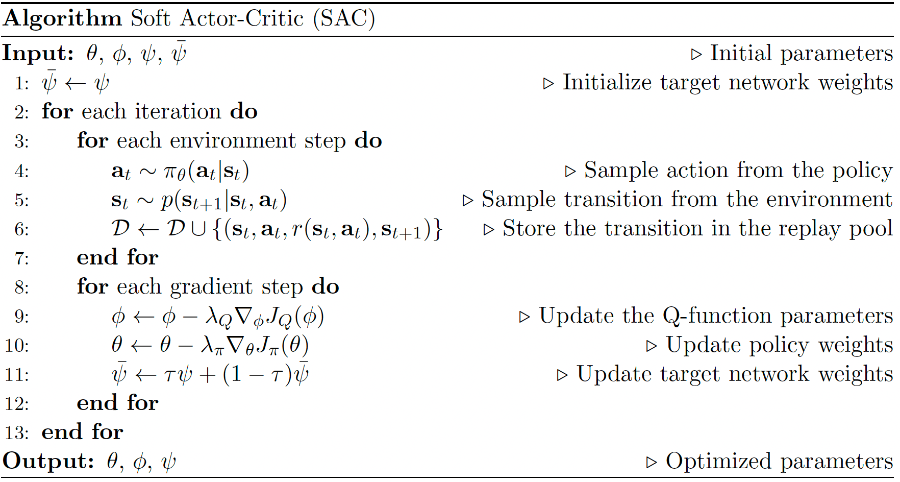
Observe that the convergence of soft policy iteration is ensured only when $\vert \mathcal{A} \vert < \infty$, constraining the application to large continuous domains. Instead of iteratively repeating evaluation and improvement to convergence, soft actor-critic (SAC) alternates between optimizing both networks with stochastic gradient descent.

SAC consists of parameterized state value function \(V_\psi (\mathbf{s}_t)\), soft Q-function \(Q_\phi (\mathbf{s}_t, \mathbf{a}_t)\) and its target value network \(V_\bar{\psi} (\mathbf{s}_t)\), and tractable actor policy \(\pi_\theta (\mathbf{a}_t \vert \mathbf{s}_t)\). (Including separate approximator for the soft value can stabilize training.)

• Soft state value $V_\psi$
  Trained to minimize the squared residual error $$ J_V (\psi) = \frac{1}{2} \mathbb{E}_{\mathbf{s}_t \sim \mathcal{D}} \left[ (V_\psi (\mathbf{s}_t) - \mathbb{E}_{\mathbf{a}_t \sim \pi_\theta} [Q_\phi (\mathbf{s}_t, \mathbf{a}_t) - \alpha \log \pi_\theta (\mathbf{a}_t \vert \mathbf{s}_t)])^2 \right] $$ where the gradient is estimated with an unbiased one-sample MC estimator $$ \nabla_{\psi} J_V (\psi) \approx \nabla_{\psi} V_\psi (\mathbf{s}_t) \times ( V_\psi (\mathbf{s}_t) - Q_\phi (\mathbf{s}_t, \mathbf{a}_t) + \alpha \log \pi_\theta (\mathbf{a}_t \vert \mathbf{s}_t) ) $$
• Soft state-action value $Q_\phi$
  Trained to minimize the soft Bellman residual $$ \begin{gathered} J_Q (\phi) = \frac{1}{2} \mathbb{E}_{(\mathbf{s}_t, \mathbf{a}_t) \sim \mathcal{D}} \left[ (Q_\phi (\mathbf{s}_t, \mathbf{a}_t) - \hat{Q}(\mathbf{s}_t, \mathbf{a}_t))^2 \right] \\ \text{ where } \hat{Q}(\mathbf{s}_t, \mathbf{a}_t) = r(\mathbf{s}_t, \mathbf{a}_t) + \gamma \mathbb{E}_{\mathbf{s}_{t+1} \sim p} [V_{\bar{\psi}} (\mathbf{s}_{t+1})] \end{gathered} $$ which again can be optimized with an unbiased one-sample MC estimator $$ \nabla_{\phi} J_Q (\phi) \approx \nabla_{\phi} Q_\phi (\mathbf{s}_t, \mathbf{a}_t) \times ( Q_\phi (\mathbf{s}_t, \mathbf{a}_t) - r(\mathbf{s}_t, \mathbf{a}_t) - \gamma V_{\bar{\psi}} (\mathbf{s}_{t+1} ) ). $$ Note that the update is based on target value network $V_{\bar{\psi}}$ which is slowly updated with exponentially moving average of the value network weights $\psi$.
• Actor $Q_\phi$
  Trained to minimize the expected KL-divergence $$ \begin{aligned} J_\pi (\theta) & = \mathbb{E}_{\mathbf{s}_t \sim \mathcal{D}} \left[ \mathrm{KL} \left( \pi_\theta (\cdot \vert \mathbf{s}_t) \Big\Vert \frac{\exp \left( \frac{1}{\alpha} Q_\phi (\mathbf{s}_t, \cdot) \right)}{Z_\phi (\mathbf{s}_t)}\right)\right] \\ & \equiv \mathbb{E}_{\mathbf{s}_t \sim \mathcal{D}, \mathbf{a}_t \sim \pi_\theta} \left[ - Q_\phi (\mathbf{s}_t, \mathbf{a}_t) + \alpha \log \pi_\theta (\mathbf{a}_t \vert \mathbf{s}_t) \right] \end{aligned} $$ Since MC approximation of the gradient of $J_\pi$ requires the sample from policy network $\pi_\theta$, which is not differentiable, the gradients can't be backpropagated through $\mathbf{a}_t$. Since the target density is the Q-function, which is represented by a neural network an can be differentiated, and it is thus convenient to apply the reparameterization trick instead of the likelihood ratio gradient estimator: $$ \mathbf{a}_t = f_\theta (\epsilon_t; \mathbf{s}_t) = \tanh (\mu_\theta (\mathbf{s}_t) + \sigma_\theta (\mathbf{s}_t) \odot \epsilon_t) $$ where $\epsilon_t \sim \mathcal{N}(\mathbf{0}, \mathbf{I})$ is an input noise vector and $\mu_\theta$ and $\sigma_\theta$ are the deterministic. This leads to the following objective $$ J_\pi (\theta) = \mathbb{E}_{\mathbf{s}_t \sim \mathcal{D}, \epsilon_t \sim \mathcal{N}} \left[ - Q_\phi (\mathbf{s}_t, f_\theta (\epsilon_t; \mathbf{s}_t)) + \alpha \log \pi_\theta (f_\theta (\epsilon_t; \mathbf{s}_t) \vert \mathbf{s}_t) \right] $$ with the one-sample MC approximation of gradient $$ \nabla_{\theta} J_\pi (\theta) \approx \alpha \nabla_{\theta} \pi (\mathbf{a}_t \vert \mathbf{s}_t) + (\alpha \nabla_{\mathbf{a}_t} \log \pi_\theta (\mathbf{a}_t \vert \mathbf{s}_t) - \nabla_{\mathbf{a}_t} Q_\phi (\mathbf{s}_t, \mathbf{a}_t)) \nabla_{\theta} f_\theta (\epsilon_t; \mathbf{s}_t) $$

$\mathbf{Fig\ 1.}$ Pseudocode for SAC.

References

[1] Wang et al., “Sample Efficient Actor-Critic with Experience Replay”, ICLR 2017.
[2] Munos et al., “Safe and Efficient Off-Policy Reinforcement Learning”, NeurIPS 2016.
[3] Remi Munos’ slides for Retrace algorithm, Google DeepMind
[4] Silver et al. “Deterministic Policy Gradient Algorithms”, PMLR 2014
[5] Lillicrap et al. “Continuous Control with Deep Reinforcement Learning”, ICLR 2016
[6] OpenAI Spinning Up, “Deep Deterministic Policy Gradient”
[7] Fujimoto et al., “Addressing Function Approximation Error in Actor-Critic Methods”, ICML 2018
[8] OpenAI Spinning Up, “TD3”
[9] Haarnoja et al., “Soft Actor-Critic: Off-Policy Maximum Entropy Deep Reinforcement Learning with a Stochastic Actor”, ICML 2018
[10] Haarnoja et al., “Soft Actor-Critic Algorithms and Applications”, arXiv:1812.05905