[RL] Offline Reinforcement Learning
While RL algorithms have been a focal point of research for decades, the integration of powerful and high-capacity function approximators, such as deep neural networks, into RL algorithms has propelled them to achieve remarkable performance across diverse domains.
The remarkable success of ML techniques in addressing a spectrum of real-world problems over the past decade largely stems from the emergence of scalable data-driven learning approaches, which continually improve with increased data exposure. It draws a wide attention to explore whether similar data-driven learning paradigms can be applied to RL objectives, thus leading to the emerge of offline reinforcement learning that leverage only previously collected offline data, without any additional online interaction.

Offline Reinforcment Learning
Formulation
Therefore, the offline RL problem can be defined as a data-driven formulation of the typical RL problem, which aims to find the optimal policy $\pi$ that maximizes the expectation of trajectory return:
\[\begin{gathered} J(\pi) = \mathbb{E}_{\tau \sim p_{\pi}} \left[ \sum_{t=0}^H \gamma^t r (\mathbf{s}_t, \mathbf{a}_t) \right] \\ \text{ where } p_{\pi} (\tau) = d_0 (\mathbf{s}_0) \prod_{t=0}^H \pi (\mathbf{a}_t \vert \mathbf{s}_t) \mathbb{P}(\mathbf{s}_{t+1} \vert \mathbf{s}_t, \mathbf{a}_t) \end{gathered}\]However, instead interacting with the environment or collecting additional transitions using the behavior policy, the learning algorithm is provided with a static dataset of transitions \(\mathcal{D} = \{ (\mathbf{s}_t^n, \mathbf{a}_t^n, r_t^n, \mathbf{s}_{t+1}^n) \vert n = 1, \cdots, N \}\), collected according to a different (unknown) behavioral policy $\mathbf{a} \sim \pi_\beta (\cdot \vert \mathbf{s})$, with state visitation frequency $\mathbf{s} \sim d^{\pi_\beta} (\cdot)$. And it aims to find an optimal policy $\pi$ that attains the largest possible cumulative reward when it is actually used to interact with the MDP.
Challenges
Offline RL is a difficult problem for multiple algorithmic challenges. While learning from a fixed dataset represents one of the primary advantages of offline RL, it also poses considerable challenges for existing online RL algorithms.
Exploration-Exploitation Dilemma
Exploration plays a pivotal role in RL and the lack of exploration can hinder agents from identifying high reward regions, or even from obtaining any reward at all, especially in scenarios where rewards are sparse. And the most obvious challenge with offline RL is that, as the training algorithm is entirely constrained to the dataset $\mathcal{D}$, there is no avenue for improving exploration, which is outside the scope of the algorithm. Consequently, if $\mathcal{D}$ lacks transitions that illustrate high-reward regions within the state space, it may be impossible to discover them.

Distributional Shift
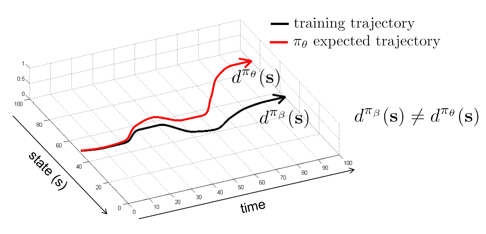
Moreover, the challenge of exploration can be further exacerbated to the well-known issue called distributional shift. While our function approximator (policy, value function, or model) may be trained under the distribution of $\mathcal{D}$, it could be evaluated and tested on a different distribution. Essentially, in such scenarios, the agent inevitably encounters out-of-distribution states, different from states on which it was trained, and the agent may make increasingly significant errors for the remainder of its trial.
Offline Approximate Dynamic Programming
Another way to optimize the RL objective involves recognizing that if we can precisely estimate value functions $V^\pi$ or $Q^\pi$, it becomes straightforward to derive a near-optimal policy. Such methodologies are well-exemplified by Q-learning and actor-critic methods, which have proven effective and are applicable to offline RL. Indeed, such techniques have been widely utilized in recent deep RL methods.
However, such methods suffer from a number of issues when only offline data is used, essentially resulting in distributional shift. Explored solutions to this issue is that one can optionally add any of the loss terms, and such approaches can be broadly grouped into three categories depending on the type of additional loss:
- policy constraint: constrain the learned policy $\pi$ to lie close to the behavior policy $\pi_{\beta}$;
- uncertainty-based: estimate the epistemic uncertainty of Q-values (e.g. from the variance), and then utilize this uncertainty to detect distributional shift;
- regularization-based: impose behaviors on the learned policy $\pi$ that do not depend on $\pi_{\beta}$ via additional penalty terms;

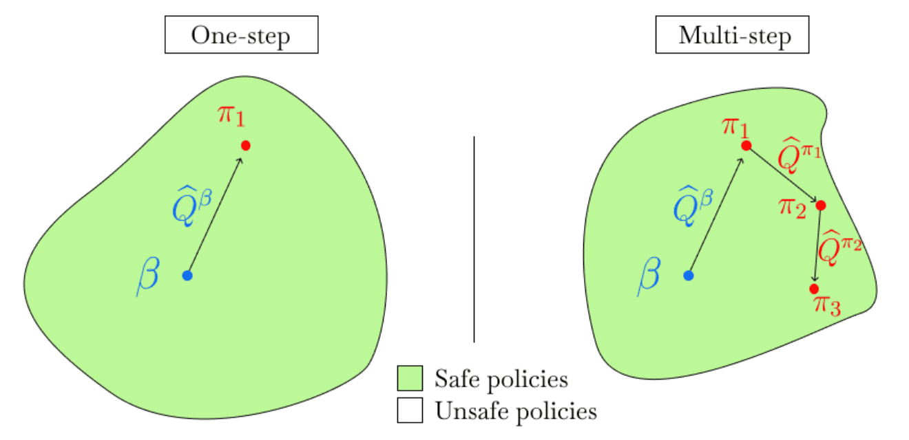
And notably, the actor–critic methods are normally implemented iteratively, alternating between policy evaluation and policy improvement steps in rapid succession. Since the agent must use an off-policy $\pi_\theta$ distinct from the behavior policy $\pi_\beta$ after a single step of policy improvement, they are susceptible to the distribution shift problem. One-step methods perform multiple state sweeps to learn an accurate estimate of $Q^\pi$, and then perform a single- policy improvement step to find the best possible policy.
Policy Constraints
Batch-Constrained Deep Q-Learning (BCQ)
One of the first policy constraint methods in offline RL was BCQ, abbreviation for batch-constrained deep Q-Learning. To mitigate the extrapolation error, a phenomenon in which unseen state-action pairs are erroneously estimated to have unrealistic values, it directly forces the learning policy $\pi_\theta$ of agent to be close to $\pi_\beta$ with a specific parameterization:
\[\pi_{\theta} (\mathbf{a} \vert \mathbf{s}) = \underset{\mathbf{a}_i + \xi_\theta (\mathbf{s}, \mathbf{a}_i)}{\arg \max} \; Q_\phi^\pi (\mathbf{s}, \mathbf{a}_i + \xi_\theta (\mathbf{s}, \mathbf{a}_i)) \text{ for } \mathbf{a}_i \sim \hat{\pi}_\beta (\cdot \vert \mathbf{s}), i = 1, \cdots, N\]where \(\hat{\pi}_\beta (\cdot \vert \mathbf{s})\) is estimated using parametric generative model (e.g. VAE) trained with supervised regression, $\xi_\theta (\mathbf{s}, \mathbf{a})$ is a perturbation model with outputs bound to a predetermined range $[−\Phi, \Phi]$, and $N$ is the number of samples.
TD3 with Behavior Cloning (TD3+BC)
Modifications to make an RL algorithm work offline comes at the cost of additional complexity. Offline RL algorithms incorporate non-algorithmic implementation changes such as new hyperparameters, and often leverage secondary components such as generative models while adjusting the underlying RL algorithm. This tends to make offline RL algorithms unstable and difficult to reproduce and tune. Moreover, such mixture of details slows down the execution times of the algorithms, and complicate causal attribution of performance improvements, as well as the transfer of techniques across different algorithms.
Fujimoto et al., 2021 simply propose to add a behavior-cloning regularizer to the policy improvement step of the TD3 algorithm, termed TD3 with Behavior Cloning (TD3+BC):
\[\begin{aligned} & \texttt{TD3}: && \pi = \underset{\pi^\prime}{\arg \max} \; \mathbb{E}_{(\mathbf{s}, \mathbf{a}) \sim \mathcal{D}} [Q (\mathbf{s}, \pi^\prime (\mathbf{s}))] \\ & \texttt{TD3+BC}: && \pi = \underset{\pi^\prime}{\arg \max} \; \mathbb{E}_{(\mathbf{s}, \mathbf{a}) \sim \mathcal{D}} [\color{red}{\lambda} Q (\mathbf{s}, \pi^\prime (\mathbf{s})) \color{red}{- (\pi^\prime (\mathbf{s}) - \mathbf{a})^2}] \end{aligned}\]where $\lambda$ controls the strength of the regularizer. By penalizing the MSE between $\pi (\mathbf{s})$ and $\mathbf{a} \sim \pi_\beta$, TD3+BC applies a form of implicit policy constraint. Technically, $\lambda$ is parameterized with tormalization term of the average absolute value of $Q$:
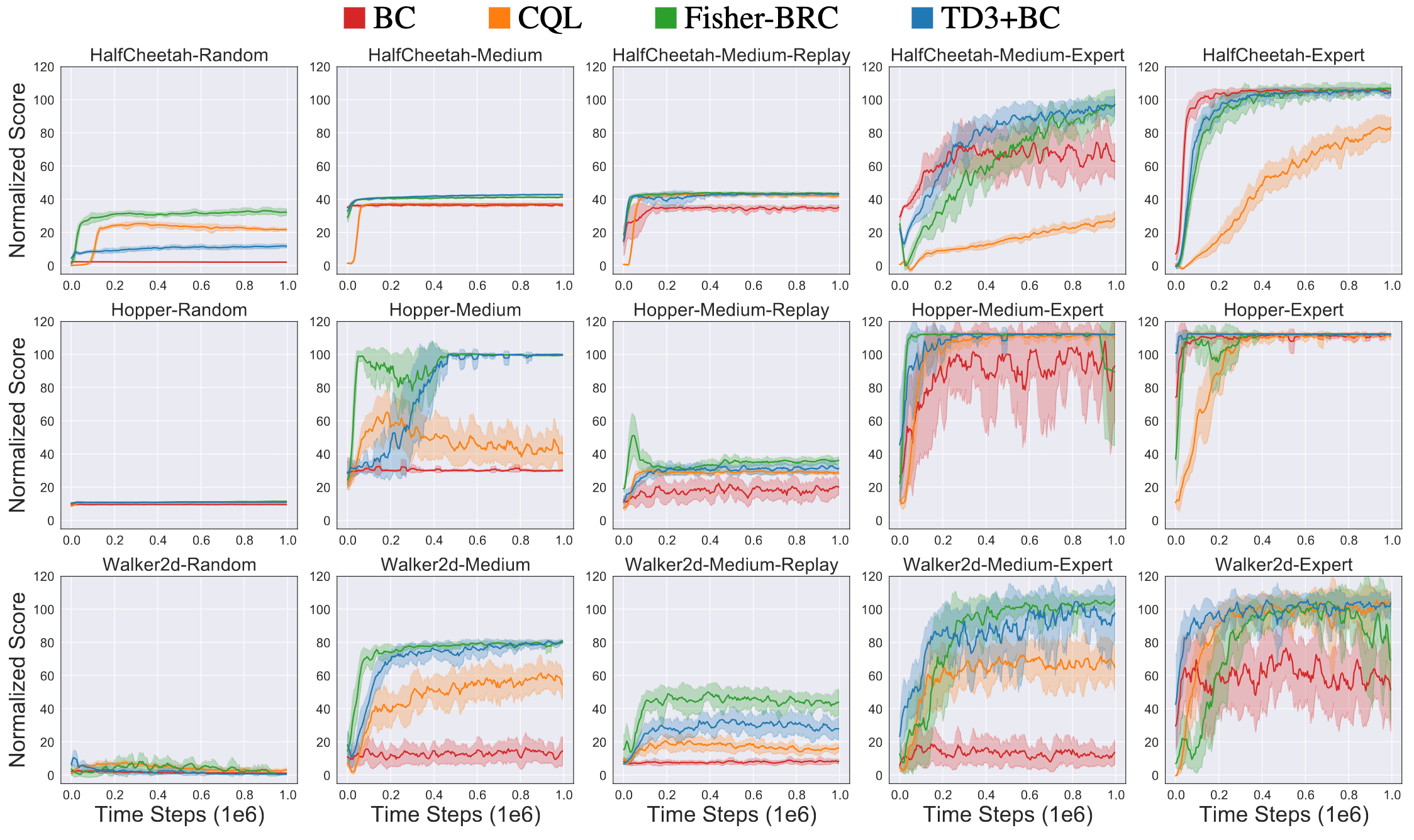
\[\lambda = \frac{\alpha}{\frac{1}{N} \sum_{(\mathbf{s}_n, \mathbf{a}_n)} Q(\mathbf{s}_n, \mathbf{a}_n)}\]provided that the balance between RL objective and imitation learning, is highly susceptible to the scale of $Q$. Practically, by only applying $z$-score normalization to the states, i.e. $\mathbf{s}_i \leftarrow \frac{\mathbf{s}_i - \mu_i}{\sigma_i + \epsilon}$ where $\mathbf{s}_i$ represents the $i$-th feature of the state $\mathbf{s}$ and ($\mu_i$, $\sigma_i$) denotes the mean and standard deviation of $\mathbf{s}_i$’s in the dataset, TD3+BC achieved competitive results with SOTA methods on various datasets, showing how performance is often not tied to algorithmic complexity.
Uncertainty Estimation
The basic intuition of the uncertainty-based methods is that if we can estimate the epistemic uncertainty of our approximations, such as the value function, or model, we expect this uncertainty to be significantly greater for out-of-distribution actions. Thus, we can use these uncertainty estimates to generate conservative target values in such cases, and we can ease the constraints on our learned policy in regions of low uncertainty, rather than restricting the policy to resemble the behavior policy.
Formally, in offline approximate dynamic programming, such methods necessitate learning an uncertainty set or distribution over possible Q-functions \(\mathbb{P}_\mathcal{D} (Q^\pi)\) from the dataset $\mathcal{D}$. Subsequently, we can improve the policy using a conservative estimate of the Q-function, which generally aligns with the following policy improvement objective with the uncertainty measure $\mathcal{U}$ (e.g., variance of \(\mathbb{P}_\mathcal{D} (Q^\pi)\)):
\[\pi_{k+1} \leftarrow \underset{\pi}{\arg \max} \; \mathbb{E}_{\mathbf{s} \sim \mathcal{D}} \underbrace{\left[\mathbb{E}_{\mathbf{a} \sim \pi(\mathbf{a} \mid \mathbf{s})}\left[\mathbb{E}_{Q_{k+1}^\pi \sim \mathcal{P}_{\mathcal{D}}\left(Q^\pi\right)}\left[Q_{k+1}^\pi(\mathbf{s}, \mathbf{a})\right]-\alpha \cdot \mathcal{U}\left(\mathbb{P}_{\mathcal{D}}\left(Q^\pi\right)\right)\right]\right]}_{\text {conservative estimate }},\]As we will explore, certain model-based methods also evaluate the learned model’s uncertainty through the use of model ensembles. These ensembles penalize out-of-distribution actions and favor decisions that are consistent across the models.
Random Ensemble Mixture (REM)
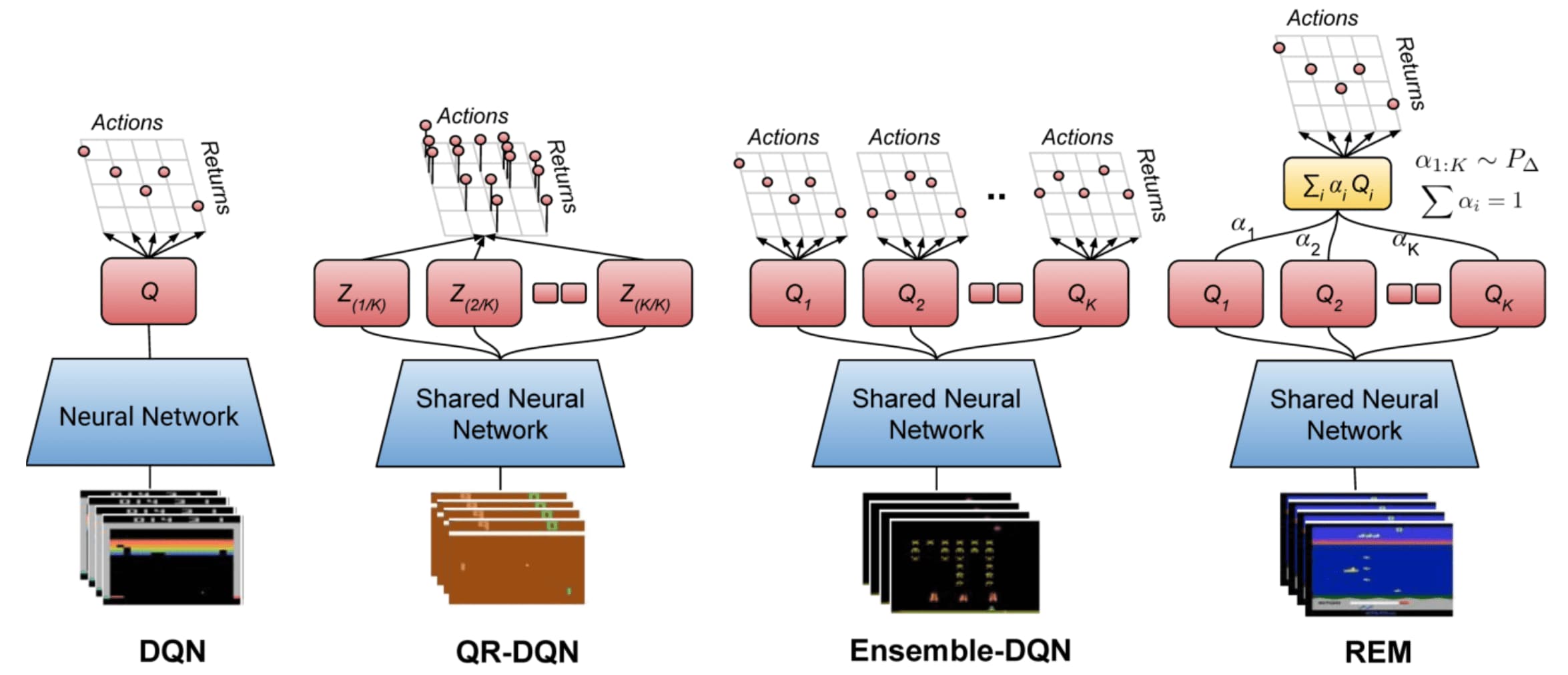
For example, Agarwal et al., 2020 proposed algorithms named ensemble-DQN and random ensemble mixture that train a sed of $K$ DQNs \(\{ Q_\theta^k (\mathbf{s}, \mathbf{a}) \}\) independently by using disjoint partitions of the dataset for each Q-function. This approach allows approximating the Q-function distribution by:
\[\mathbb{P}_\mathcal{D} (Q^\pi) \approx \frac{1}{K} \sum_{k=1}^K \delta \left[ Q^\pi = Q_\theta^k \right]\]and the Q-function itself by random convex combination, in case of REM:
\[\begin{gathered} Q^\pi (\mathbf{s}, \mathbf{a}) \approx \sum_{k=1}^K \alpha_k \cdot Q_\theta^k (\mathbf{s}, \mathbf{a}) \\ \text{ s.t. } \sum_{k=1}^K \alpha_k = 1 \text{ and } \alpha_k = \frac{\alpha_k^\prime}{\sum_j \alpha_j^\prime} \text{ where } \alpha_j^\prime \sim U(0, 1) \end{gathered}\]
Regularization
Policy Regularization: Soft Actor-Critic (SAC)
Soft Actor-Critics (SACs), proposed by Haarnoja et al., 2018, introduced an entropy regularization term to the policy gradient objective to enforce the policy to explore more broadly, making possible to capture mutliple modes of near-optimal behavior.
\[\pi^* = \underset{\pi}{\arg \max} \; \mathbb{E}_{\tau \sim \pi} \left[ \sum_{t=0} \gamma^t \Big( r (\mathbf{s}_t, \mathbf{a}_t) + \alpha \mathbb{H}[\pi (\cdot \vert \mathbf{s}_t)] \Big) \right] \text{ where } \mathbb{H}(\mathbb{P}) = \mathbb{E}_{\mathbf{x} \sim \mathbb{P}} [ - \log \mathbb{P}(\mathbf{x}) ]\]By adjusting the weight to the regularization term, the more stochastic we wish the policy to be.
Value Regularization: Conservative Q-Learning (CQL)
The policy $\pi$ of value-based off-policy algorithms is trained to maximize Q-values. In an offline setting, this generally yield poor performance due to overestimated, optimistic value function estimates attributed by bootstrapping from out-of-distribution actions and overfitting. Recall that the general loss function of value-based off-policy RL is defined as follows for target policy $\pi$:
\[\texttt{General Offline RL: } \mathcal{J} (\theta) = \mathbb{E}_{(\mathbf{s}, \mathbf{a}, \mathbf{s}^\prime) \sim \mathcal{D}} \left[\left( r(\mathbf{s}, \mathbf{a}) + \gamma \mathbb{E}_{\mathbf{a}^\prime \sim \pi (\cdot \vert \mathbf{s})} [Q_\theta (\mathbf{s}^\prime, \mathbf{a}^\prime)] - Q_\theta (\mathbf{s}, \mathbf{a}) \right)^2 \right]\]
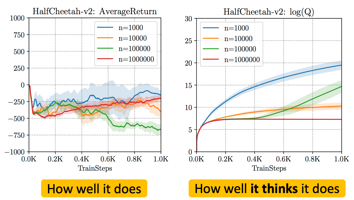
Instead, intuitively, by learning a conservative estimate of the value function that offers a lower bound on the true values, this overestimation problem can be mitigated. Conservative Q-Learning (CQL) simply learns such “conservative” Q-functions by just adding regularization terms $\mathcal{R}(\theta)$:
\[\texttt{Conservative Q-Learning: } \mathcal{L} (\theta) = \mathcal{J} (\theta) + \mathcal{R}(\theta)\]where
\[\begin{aligned} \mathcal{R} (\theta) = & \max_{\mu} \mathbb{E}_{\mathbf{s} \sim \mathcal{D}, \mathbf{a} \sim \mu (\cdot \vert \mathbf{s})} [Q_\theta (\mathbf{s}, \mathbf{a})] \\ & - \mathbb{E}_{\mathbf{s} \sim \mathcal{D}, \mathbf{a} \sim \pi_\beta (\cdot \vert \mathbf{s})} [Q_\theta (\mathbf{s}, \mathbf{a})] + \mathcal{R} (\mu) \end{aligned}\]and $\mathcal{R} (\mu)$ is a regularization term for the policy $\mu (\mathbf{a} \vert \mathbf{s})$. It minimizes values under an appropriately chosen distribution $\mu (\cdot \vert \mathbf{s})$ that visits the unseen actions in $\mathcal{D}$ (that is, out-of-distribution of $\pi_\beta$), and then further tightening this bound by also incorporating a maximization term over the data distribution.
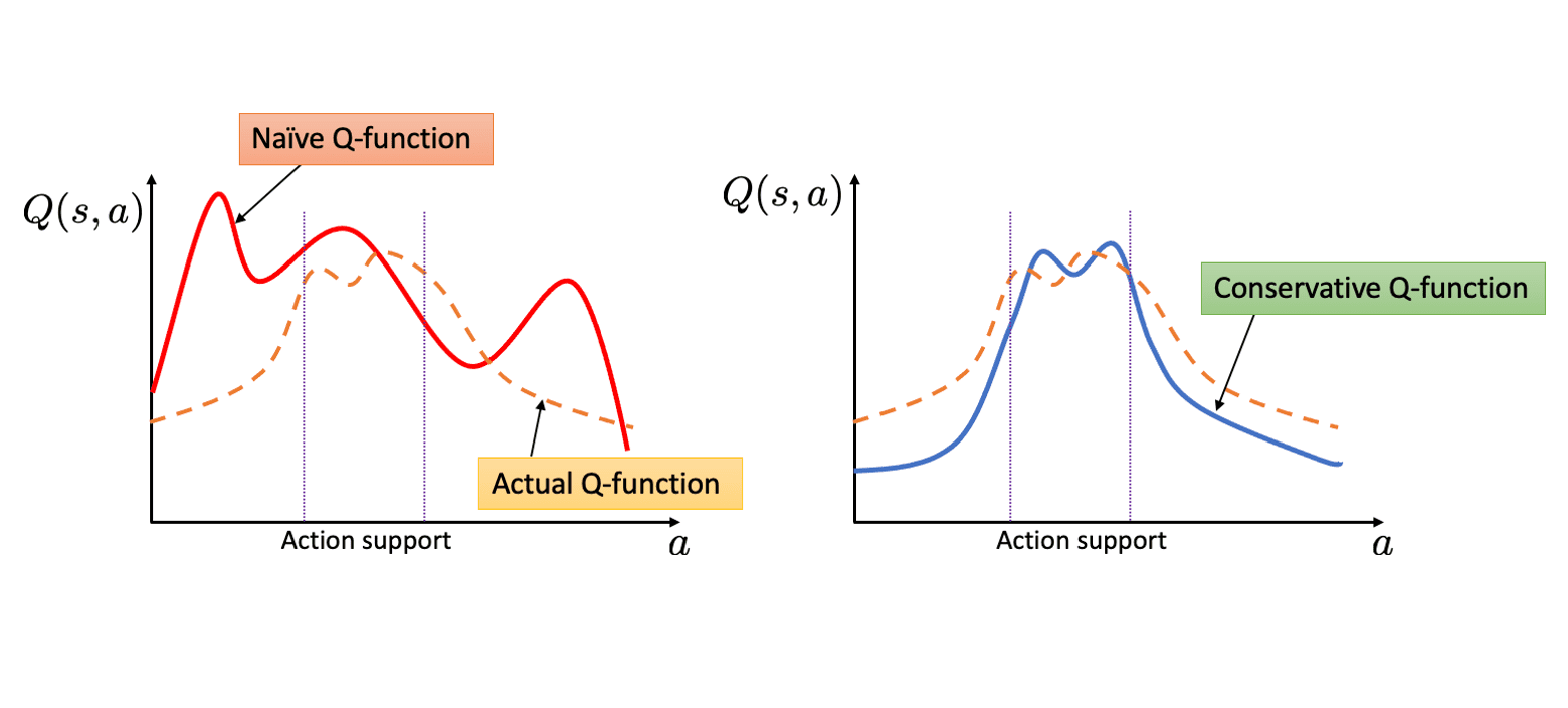
The authors theoretically demonstrated that CQL underestimates the value function at every state in the dataset $\mathcal{D}$ if the mild regularity conditions hold (slow updates on the policy):
\[\forall \mathbf{s} \in \mathcal{D}: \; \hat{V}_{\texttt{CQL}}^\pi (\mathbf{s}) \leq V^\pi (\mathbf{s})\]One-step Methods
Many deep offline RL algorithms rely on an actor-critic framework, alternating between policy evaluation and policy improvement steps over multiple iterations (multi-step methods). Since the agent must use an off-policy $\pi_\theta$ distinct from the behavior policy $\pi_\beta$ after a single step of policy improvement, it is well-known that they are susceptible to the distribution shift problem.
To address the issue, explicit constraints such as regularization (e.g., SAC, CQL) or penalty terms (e.g., BCQ, TD3+BC) can be supplemented to restrict the agent policy $\pi_\theta$ to remain within the “safe” region around the behavior policy $\pi_\beta$. Nevertheless, querying or estimating values for unseen actions remains vulnerable to misestimation.
\[\texttt{General Offline RL: } \mathcal{L}(\theta) = \mathbb{E}_{(\mathbf{s}, \mathbf{a}, \mathbf{s}^\prime) \sim \mathcal{D}} \left[ \left( r (\mathbf{s}, \mathbf{a}) + \gamma \color{blue}{\max_{\mathbf{a}^\prime \in \mathcal{A}}} Q_{\hat{\theta}} (\mathbf{s}^\prime, \mathbf{a}^\prime) - Q_\theta (\mathbf{s}, \mathbf{a}) \right)^2 \right]\]

Implicit Q-Learning (IQL)
Implicit Q-Learning (IQL) is one of the most representative works in one-step methods that learns the optimal policy wihtout directly querying or estimating values for unseen actions, but with implicit constraints using advantage-weighted behavioral cloning.
\[\texttt{IQL: } \mathcal{L}(\theta) = \mathbb{E}_{(\mathbf{s}, \mathbf{a}, \mathbf{s}^\prime) \sim \mathcal{D}} \left[ \left( r (\mathbf{s}, \mathbf{a}) + \gamma \color{red}{\max_{\begin{gathered} \mathbf{a}^\prime \in \mathcal{A} \\ \text{ s.t. } \pi_\beta (\mathbf{a}^\prime \vert \mathbf{s}^\prime) > 0 \end{gathered}}} Q_{\hat{\theta}} (\mathbf{s}^\prime, \mathbf{a}^\prime) - Q_\theta (\mathbf{s}, \mathbf{a}) \right)^2 \right]\]To do so, IQL performs a single step of policy evaluation to learn an accurate estimate of $Q^{\pi_\beta} (\mathbf{s}, \mathbf{a})$, followed by a single-policy improvement step (one-step methods) to extract the best policy at once.
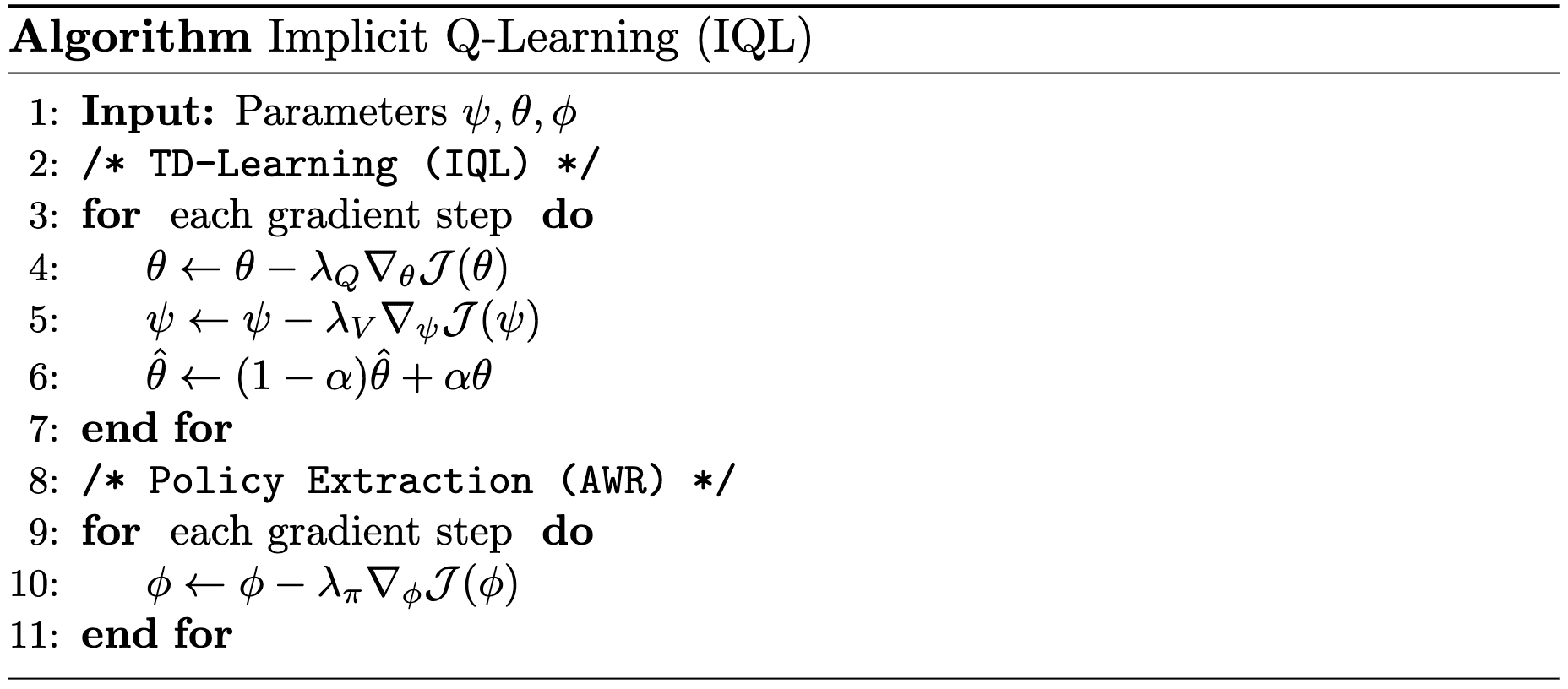
TD-Learning (IQL)
To avoid querying or estimating the values for unseen actions, implicit Q-learning leverages a function approximator $V_\psi$ for $V^\pi$ as the target, instead of using target actions sampled from $\mathbf{a}^* \sim \pi_\beta (\cdot \vert \mathbf{s}^\prime)$:
\[J(\theta) = \mathbb{E}_{(\mathbf{s}, \mathbf{a}, \mathbf{s}^\prime) \sim \mathcal{D}} [r (\mathbf{s}, \mathbf{a}) + V_\psi (\mathbf{s}^\prime) - Q_\theta (\mathbf{s}, \mathbf{a})]\]To ensure the above update is meaningful, $V_\psi (\mathbf{s})$ should converge to $\max_{\mathbf{a} \in \mathcal{A}} Q_\theta (\mathbf{s}, \mathbf{a})$. Therefore, IQL also optimizes the following objective:
\[\mathcal{J} (\psi) = \mathbb{E}_{(\mathbf{s}, \mathbf{a}) \sim \mathcal{D}} [\mathcal{L} (Q_{\hat{\theta}} (\mathbf{s}, \mathbf{a}) - V_\psi (\mathbf{s}))]\]for some loss metric $\mathcal{L} (\cdot)$ where $Q_\hat{\theta}$ is the target network, i.e., the EMA version of Q-network $Q_\theta$. For example, observe that the minimizer of the objective is \(V_\psi^* (\mathbf{s}) = \mathbb{E}_{\mathbf{a} \sim \pi_\beta (\cdot \vert \mathbf{s})} [Q_\theta (\mathbf{s}, \mathbf{a})]\) if $\mathcal{L}$ is set to MSE loss, aligning with the Bellman equations.
And the authors demonstrated that expectile regression (\(\mathcal{L}_2^\tau\) for $\mathcal{L}$) by setting larger values for $\tau$ allows us to satisfy the Bellman optimality equations, i.e., \(V_\psi^* (\mathbf{s}) = \max_{\mathbf{a} \in \mathcal{A}} Q_\theta (\mathbf{s}, \mathbf{a})\):
\[\begin{gathered} \mathcal{J} (\psi) = \mathbb{E}_{(\mathbf{s}, \mathbf{a}) \sim \mathcal{D}} [\mathcal{L}_2^\tau (Q_\hat{\theta} (\mathbf{s}, \mathbf{a} - V_\psi (\mathbf{s})))] \\ \text{ where } \mathcal{L}_2^\tau (u) = \vert \tau - \mathbf{1}(u < 0) \vert u^2 \end{gathered}\]The authors theoretically proved that the minimizer $V_\tau$ of the above loss is the best value from the actions within the support of dataset $\mathcal{D}$:
\[\lim_{\tau \to 1} V_\tau (\mathbf{s}) = \max_{\begin{gathered} \mathbf{a} \in \mathcal{A} \\ \text{ s.t. } \pi_\beta (\mathbf{a} \vert \mathbf{s}) > 0 \end{gathered}} Q^* (\mathbf{s}, \mathbf{a})\]Policy Extraction
After learning values by policy improvement steps, the policy $\pi_\phi$ is extracted using advantage weighted regression (AWR) with EMA version of Q-function $Q_\hat{\theta}$:
\[\mathcal{J} (\phi) = \mathbb{E}_{(\mathbf{s}, \mathbf{a}) \sim \mathcal{D}}[ \exp \left( \beta ( Q_{\hat{\theta}}(\mathbf{s}, \mathbf{a}) - V_\psi (\mathbf{s})) \right) \log \pi_\phi (\mathbf{a} \vert \mathbf{s})]\]where $\beta \in [0, \infty)$ is an inverse temperature.
Offline Model-Based RL
Direct application of MBRL algorithms to offline settings can be problematic due to the distribution shifts and the inability of offline-learned models to correct errors through environmental interaction. Since the offline dataset may not cover the entire state-action space, the learned models are unlikely to be globally accurate. Consequently, planning with the learned model without any safeguards against model inaccuracy can result in model exploitation, yielding poor results. In this post, we explore some previous efforts to adapt MBRL for offline setting.
Model-Based Offline RL (MOReL)
Kidambi et al., 2020 proposed a method named model-based offline RL (MOReL) that consists of two modular steps:
- Learning pessimistic MDP (P-MDP) with the offline dataset
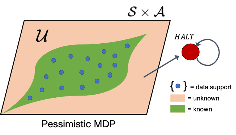
The P-MDP partitions the state space into "known" and "unknown" regions, and uses a large negative reward for unknown regions. This provides a regularizing effect during policy learning by heavily penalizing policies that visit unknown states. In contrast, model-free algorithms are forced to regularize the policies directly towards the data logging policy, which can be overly conservative. - Learning near-optimal policy for the P-MDP
For any policy, the performance in the true MDP (real environment) is approximately lower-bounded by the performance in the P-MDP. making it a suitable surrogate for purposes of policy evaluation and learning, and overcome common pitfalls of model-based RL like model exploitation.

To partition the state-action space into known and unknown regions, they proposed a measure of disagreement between the true dynamics and learned model:
Let $\hat{\mathbb{P}}(\cdot \vert \mathbf{s}, \mathbf{a})$ be an approximate dynamics model of the true dynamics $\mathbb{P}(\cdot \vert \mathbf{s}, \mathbf{a})$. Given a state-action pair $(\mathbf{s}, \mathbf{a})$, define an unknown state action detector as: $$ U^\alpha (\mathbf{s}, \mathbf{a}) = \begin{cases} \textrm{FALSE (i.e. Known)} & \mathrm{if} \quad \mathrm{TV} \left( \hat{\mathbb{P}}(\cdot \vert \mathbf{s}, \mathbf{a}), \mathbb{P}(\cdot \vert \mathbf{s}, \mathbf{a}) \right) \leq \alpha \text{ can be guaranteed} \\ \textrm{TRUE (i.e. Unknown)} & \mathrm{otherwise} \end{cases} $$
Then, a pessimistic MDP (P-MDP) can be constructed using the learned model and USAD by penalizing policies that venture into unknown parts of state-action space:
The $(\alpha, \kappa)$-pessimistic MDP $\hat{\mathcal{M}}_p$ is described by a set of tuples: $$ \hat{\mathcal{M}}_p := \{ S \cup \texttt{HALT}, A, r_p, \hat{\mathbb{P}}_p, \hat{\rho}_0, \gamma \} $$
- $(S, A)$ are states and actions in the true MDP (environment) $\mathcal{M}$.
- $\texttt{HALT}$ is an additional absorbing state.
- $\hat{\rho}_0$ is the initial state distribution learned from the dataset $\mathcal{D}$.
- $\gamma$ is the discount factor (same as $\mathcal{M}$).
- The modified reward and transition dynamics are given by: $$ \begin{split} \hat{\mathbb{P}}_{p}(\mathbf{s}^\prime \vert \mathbf{s}, \mathbf{a}) = \begin{cases} \delta(\mathbf{s}^\prime=\texttt{HALT}) & \begin{array}{l} \mathrm{if} \; U^\alpha(\mathbf{s}, \mathbf{a}) = \mathrm{TRUE} \\ \mathrm{or} \; \mathbf{s} = \texttt{HALT} \end{array} \\ \hat{\mathbb{P}}(\mathbf{s}^\prime \vert \mathbf{s}, \mathbf{a}) & \mathrm{otherwise} \end{cases} \end{split} \quad \begin{split} r_p (\mathbf{s}, \mathbf{a}) = \begin{cases} -\kappa & \mathrm{if} \; \mathbf{s} = \texttt{HALT} \\ r(\mathbf{s}, \mathbf{a}) & \mathrm{otherwise} \end{cases} \end{split} $$ That is, the P-MDP forces the original MDP to transition to the absorbing state $\texttt{HALT}$ for unknown state-action pairs. And unknown state-action pairs are penalized by a negative reward of $−\kappa$, while all known state-actions receive the same reward as in the environment.
In the practical implementation, the uncertainty distance of USAD (i.e., TV distance) is approximated by the predictions of ensembles of models \(\{ f_{\phi_1}, f_{\phi_2}, \cdots \}\) where each model uses a different weight initialization and are optimized with different mini-batch sequences:
\[\texttt{disc} (\mathbf{s}, \mathbf{a}) = \max_{i, j} \Vert f_{\phi_i} (\mathbf{s}, \mathbf{a}) - f_{\phi_j} (\mathbf{s}, \mathbf{a}) \Vert_2\]That is, the practical $\alpha$-USAD is given by:
\[U_{\texttt{practical}}^\alpha (\mathbf{s}, \mathbf{a}) = \begin{cases} \textrm{FALSE (i.e. Known)} & \mathrm{if} \quad \texttt{disc} (\mathbf{s}, \mathbf{a}) \leq \mathrm{threshold} \\ \textrm{TRUE (i.e. Unknown)} & \mathrm{otherwise} \end{cases}\]After defining P-MDP, the final step in MOReL is to perform planning within the P-MDP that provides a good safeguards against the inaccurate and unknown regions of the learned model, which may cause distribution shift and model exploitation, extracting the final policy $\pi_{\texttt{out}}$.

Although the P-MDP is pessimistic in the sense that it only offers validated $(\mathbf{s}, \mathbf{a})$ pairs to the agent, the authors demonstrated that it serves as a suitable approximation of the MDP, thereby effectively transferring its learning progress to the actual environment.
The value of any policy $\pi$ on the original MDP $\mathcal{M}$ and its $(\alpha, R_{\max})$-pessimistic MDP $\hat{\mathcal{M}}_p$ satisfies: $$ \begin{aligned} \mathcal{J}_{\hat{\rho}_0}(\pi, \hat{\mathcal{M}}_p) &\geq \mathcal{J}_{\rho_0}(\pi, \mathcal{M}) - \frac{2 R_{\max}}{1-\gamma} \cdot \mathrm{TV}(\rho_0, \hat{\rho}_0) - \frac{2 \gamma R_{\max}}{(1-\gamma)^2} \cdot \alpha - \frac{2 R_{\max}}{1-\gamma} \cdot \mathbb{E}\left[\gamma^{\mathcal{T}_\mathcal{U}^\pi}\right] \\ \mathcal{J}_{\hat{\rho}_0}(\pi, \hat{\mathcal{M}}_p) &\leq \mathcal{J}_{\rho_0}(\pi, \mathcal{M}) + \frac{2 R_{\max}}{1-\gamma} \cdot \mathrm{TV}(\rho_0, \hat{\rho}_0) + \frac{2 \gamma R_{\max}}{(1-\gamma)^2}\cdot \alpha \end{aligned} $$ where $\mathcal{T}_\mathcal{U}^\pi$ denotes the hitting time of unknown states by $\pi$ on $\mathcal{M}$: $$ \mathcal{U} = \{ (\mathbf{s}, \mathbf{a}) \vert U^\alpha (\mathbf{s}, \mathbf{a}) = \mathrm{TRUE} \} $$ and $\mathcal{J}$ is the expected performance on the environment with states sampled according to $\rho_0$: $$ \mathcal{J}_{\rho_0} (\pi, \mathcal{M}) = \mathbb{E}_{\mathbf{s} \sim \rho_0} [V_\pi (\mathbf{s}, \mathcal{M})] \text{ where } V_\pi (\mathbf{s}, \mathcal{M}) = \mathbb{E} \left[ \sum_{t=0}^\infty \gamma^t r(\mathbf{s}_t, \mathbf{a}_t) \middle\vert \mathbf{s}_0 = \mathbf{s} \right] $$
Model-Based Policy Optimization (MOPO)
Similar to MOReL, model-based offline policy optimization (MOPO) by Yu et al., 2020 also optimizes a policy in an uncertainty-penalized MDP, where the reward function is penalized by an estimate $u (\mathbf{s}, \mathbf{a})$ of the model’s error. This safe MDP theoretically enables the agent to maximize a lower bound of the return in the true MDP.
Unlike MOReL, which constructs terminating states $\texttt{HALT}$ based on a hard threshold on uncertainty, MOPO uses a soft reward penalty to incorporate uncertainty. Specifically, MOPO quantifies the uncertainty as the maximum $\Vert \cdot \Vert_F$ among the ensemble of multivariate Gaussian dynamic models \(\hat{\mathbb{P}}_{\theta, \phi}^i (\mathbf{s}^\prime \vert \mathbf{s}, \mathbf{a}) = \mathcal{N}(\mu_\theta^i (\mathbf{s}, \mathbf{a}), \Sigma_\phi^i (\mathbf{s}, \mathbf{a}))\):
\[\begin{aligned} & \texttt{MOReL: } \tilde{r}(\mathbf{s}, \mathbf{a}) = \begin{cases} r(\mathbf{s}, \mathbf{a}) & \mathrm{if} \; \max_{i, j} \Vert f_{\phi_i} (\mathbf{s}, \mathbf{a}) - f_{\phi_j} (\mathbf{s}, \mathbf{a}) \Vert_2 \leq \alpha \\ - R_{\max} & \mathrm{otherwise} \end{cases} \\ & \\ & \texttt{MOPO: } \tilde{r}(\mathbf{s}, \mathbf{a}) = r (\mathbf{s}, \mathbf{a}) - \lambda \max_{1 \leq i \leq N} \Vert \Sigma_\phi^i (\mathbf{s}, \mathbf{a}) \Vert_F \end{aligned}\]Given an error estimator $u (\mathbf{s}, \mathbf{a})$, the uncertainty-penalized MDP is defined as follows:
The uncertainty-penalized MDP $\widetilde{\mathcal{M}}$ is defined by tuple $(\mathcal{S}, \mathcal{A}, \hat{\mathbb{P}}, \tilde{r}, \mu_0, \gamma)$ where $\hat{\mathbb{P}}$ is the learned dynamics and $\tilde{r}$ is the uncertainty-penalized reward: $$ \tilde{r} (\mathbf{s}, \mathbf{a}) := r(\mathbf{s}, \mathbf{a}) - \lambda u (\mathbf{s}, \mathbf{a}) $$
Under some assumptions, they theoretically proved that the uncertainty-penalized MDP $\widetilde{\mathcal{M}}$ is conservative in that the return under it bounds from below the true return:
\[\mathcal{J} (\pi, \mathcal{M}) \geq \mathcal{J} (\pi, \widetilde{\mathcal{M}})\]In practical implementation, the dynamics are approximated by networks that outputs Gaussian parameters $\mu_\theta$ and $\Sigma_\phi$, yielding:
\[\hat{\mathbb{P}}_{\theta, \pi} (\mathbf{s}_{t+1}, r \vert \mathbf{s}_t, \mathbf{a}_t) = \mathcal{N} (\mu_\theta (\mathbf{s}_t, \mathbf{a}_t), \Sigma_\phi (\mathbf{s}_t, \mathbf{a}_t))\]To design the uncertainty estimator that captures both the epistemic and aleatoric uncertainty of the true dynamics, the MOPO learns an ensemble of $N$ dynamics models with each model trained independently via maximum likelihood:
\[\{\hat{\mathbb{P}}_{\theta, \pi}^i = \mathcal{N} (\mu_\theta^i, \Sigma_\phi^i) \}_{i=1}^N\]and error estimator $u(\mathbf{s}, \mathbf{a})$ is designed using the learned variance of Gaussian:
\[u(\mathbf{s}, \mathbf{a}) = \max_{i=1, \cdots, N} \Vert \Sigma_\phi^i (\mathbf{s}, \mathbf{a}) \Vert_F\]Although this lacks theoretical guarantees, the authors found that it is sufficiently accurate to achieve good performance in practice. After defining uncertainty-penalized MDP, MOPO perform policy-optimization within that MDP, extracting the final policy $\hat{\pi}$.

Define the expected error $\varepsilon_u (\pi)$ of the model accumulated along trajectories induced by $\pi$: $$ \varepsilon_u (\pi) := \mathbb{E}_{(\mathbf{s}, \mathbf{a}) \sim \rho_{\hat{\mathbb{P}}}^\pi} \left[ u (\mathbf{s}, \mathbf{a}) \right] $$ Assume that:
- We can represent the value function with $\mathcal{F}$
For any policy $\pi$, $V_\mathcal{M}^\pi \in c \mathcal{F}$ for some scalar $c \in \mathbb{R}$. - The model error is bounded above by $u (\mathbf{s}, \mathbf{a})$
$u$ is an admissible estimator for learned dynamics $\hat{\mathbb{P}}$ in the sense that: $$ \forall (\mathbf{s}, \mathbf{a}) \in \mathcal{S} \times \mathcal{A}: \quad d_\mathcal{F} (\hat{\mathbb{P}} (\cdot \vert \mathbf{s}, \mathbf{a}), \mathbb{P} (\cdot \vert \mathbf{s}, \mathbf{a})) \leq u(\mathbf{s}, \mathbf{a}) $$
Conservative Offline Model-Based Policy Optimization (COMBO)
Prior model-based offline RL approaches necessitate uncertainty quantification for incorporating conservatism, which is challenging and often unreliable in practice. For instance, uncertainty quantification is hard in these tasks where the agent is required to go further away from the data distribution.
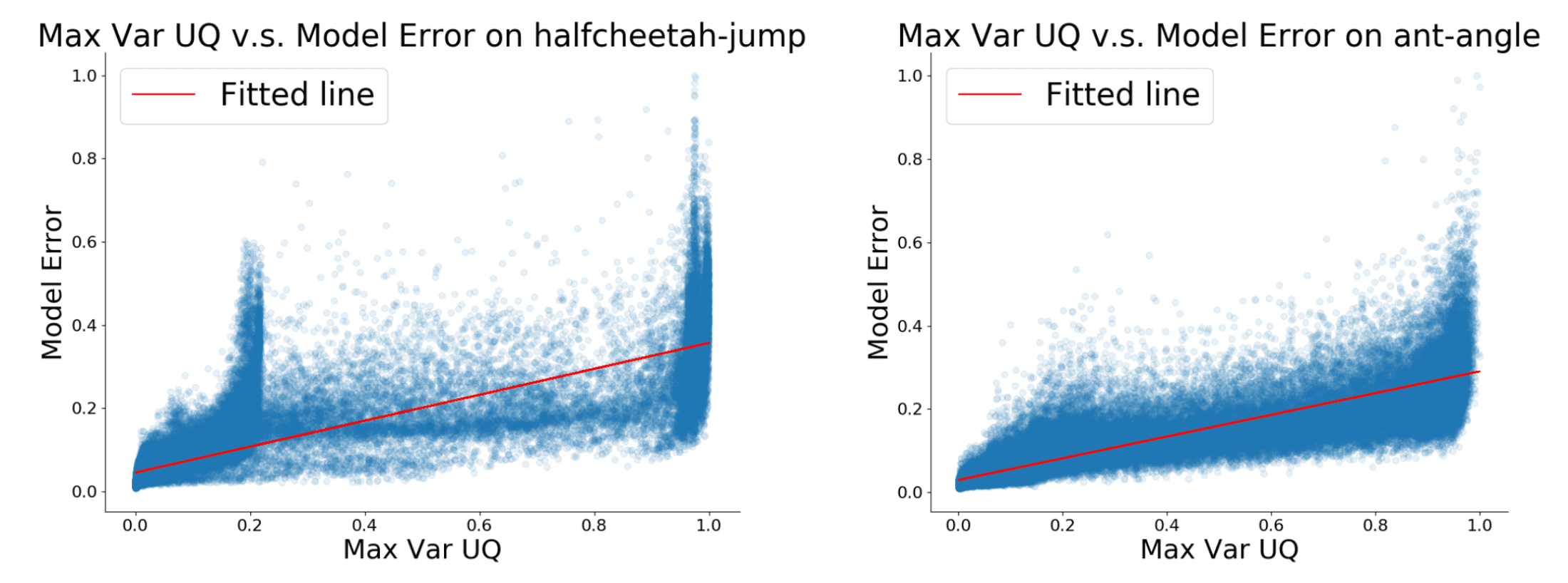
Instead of integrating conservatism into model dynamics, Yu et al., NeurIPS 2021 introduced a model-based version of CQL named conservative offline model-based policy optimization (COMBO), which incorporates conservatism into policy learning without uncertainty estimation.
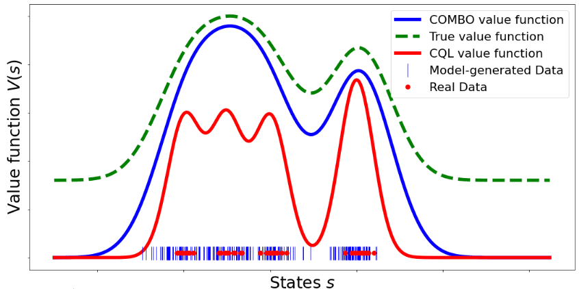
COMBO also learns a single Gaussian dynamics model $\hat{\mathbb{P}} (\mathbf{s}^\prime, r \vert \mathbf{s}, \mathbf{a}) = \mathcal{N}(\mu_\theta (\mathbf{s}, \mathbf{a}), \Sigma_\theta (\mathbf{s}, \mathbf{a}))$ via maximum log-likelihood. With both the offline dataset and simulated data from the model, it learns a conservative (but less than CQL) critic function by penalizing the value function in state-action tuples that are not in the support of the offline dataset.
Given a policy $\pi$, an offline dataset $\mathcal{D}$, and a learned model $\hat{\mathcal{M}}$ of the MDP, COMBO obtains a conservative estimate of $Q^\pi$ by penealizing the Q-values evaluated on data drawn from a particular state-action distribution that is more likely to be out-of-support while pushing up the Q-values on state-action pairs that are trustworthy, which is implemented by repeating the following recursion:
\[\begin{multline} \hat{Q}^{k + 1} \leftarrow \underset{Q}{\arg \min} \; \alpha \left( \mathbb{E}_{\mathbf{s} \sim d_{\hat{\mathcal{M}}}^\pi, \mathbf{a} \sim \pi (\cdot \vert \mathbf{s})} [Q (\mathbf{s}, \mathbf{a})] - \mathbb{E}_{(\mathbf{s} , \mathbf{a}) \sim \mathcal{D}} [Q (\mathbf{s}, \mathbf{a})] \right) \\ + \frac{1}{2} \mathbb{E}_{(\mathbf{s}, \mathbf{a}, \mathbf{s}^\prime) \sim d_f^\mu} \left[ \left( r (\mathbf{s}, \mathbf{a}) + \gamma \hat{Q}^k (\mathbf{s}^\prime, \mathbf{a}^\prime) - Q(\mathbf{s}, \mathbf{a}) \right)^2 \right] \end{multline}\]where \(d_{\hat{\mathcal{M}}}^\pi(\mathbf{s})\) is the discounted marginal state distribution when executing $\pi$ in the learned model $\hat{\mathcal{M}}$, and $d_f$ is an $f \in [0, 1]$−interpolation between the offline dataset and synthetic rollouts from the model:
\[d_f^\mu (\mathbf{s}, \mathbf{a}) := f \cdot d (\mathbf{s}, \mathbf{a}) + (1 - f) \cdot d_{\hat{\mathcal{M}}}^\mu (\mathbf{s}, \mathbf{a})\]for the rollout distribution $\mu (\mathbf{a} \vert \mathbf{s})$. After learning a conservative critic $\hat{Q}^\pi$, we can improve the policy as:
\[\pi^\prime \leftarrow \underset{\pi}{\arg \max} \; \mathbb{E}_{\mathbf{s} \sim d_{\hat{\mathcal{M}}}^\pi, \mathbf{a} \sim \pi (\cdot \vert \mathbf{s})} \left[ \hat{Q}^\pi (\mathbf{s}, \mathbf{a}) \right]\]

The authors proved that COMBO is less conservative in that it does not underestimate the value function at every state in the dataset like CQL:
\[\forall \mathbf{s} \in \mathcal{D}: \; \hat{V}_{\texttt{CQL}}^\pi (\mathbf{s}) \leq V^\pi (\mathbf{s})\]whereas the COMBO bound is only valid in expectation of the value function over the initial state distribution and the value function at a given state may not be a lower-bound:
\[\mathbb{E}_{\mathbf{s} \sim \mu_0 (\mathbf{s})} \left[ \hat{V}_{\texttt{COMBO}}^\pi (\mathbf{s}) \right] \leq \mathbb{E}_{\mathbf{s} \sim \mu_0 (\mathbf{s})} \left[ V^\pi (\mathbf{s}) \right]\]References
[1] Levine et al., “Offline Reinforcement Learning: Tutorial, Review, and Perspectives on Open Problems”, NeurIPS 2020 Tutorial
[2] A Survey on Offline Reinforcement Learning: Taxonomy, Review, and Open Problems Rafael Figueiredo Prudencio , Marcos R. O. A. Maximo , and Esther Luna Colombini , Member, IEEE
[3] Fujimoto et al., “Off-policy Deep Reinforcement Learning without Exploration”, ICML 2019
[4] Fujimoto et al., “A Minimalist Approach to Offline Reinforcement Learning”, NeurIPS 2021 Spotlight
[5] Agarwal et al., “An Optimistic Perspective on Offline Reinforcement Learning”, ICML 2020
[6] Haarnoja et al., “Soft Actor-Critic: Off-Policy Maximum Entropy Deep Reinforcement Learning with a Stochastic Actor”, ICML 2018
[7] Haarnoja et al., “Soft Actor-Critic Algorithms and Applications”, arXiv:1812.05905
[8] Kumar et al., “Conservative Q-Learning for Offline Reinforcement Learning”, NeurIPS 2020
[9] Kostrikov et al., “Offline Reinforcement Learning with Implicit Q-Learning”, ICLR 2022 Poster
[10] Brandfonbrener et al., “Offline RL Without Off-Policy Evaluation”, NeurIPS 2021
[11] Kidambi et al., “MOReL: Model-Based Offline Reinforcement Learning”, NeurIPS 2020
[12] Yu et al., “MOPO: Model-based Offline Policy Optimization”, NeurIPS 2020
[13] Yu et al., “COMBO: Conservative Offline Model-Based Policy Optimization”, NeurIPS 2021

Leave a comment