[RL] Implicit Q-Learning (IQL)

Motivation: One-step v.s. Multi-step

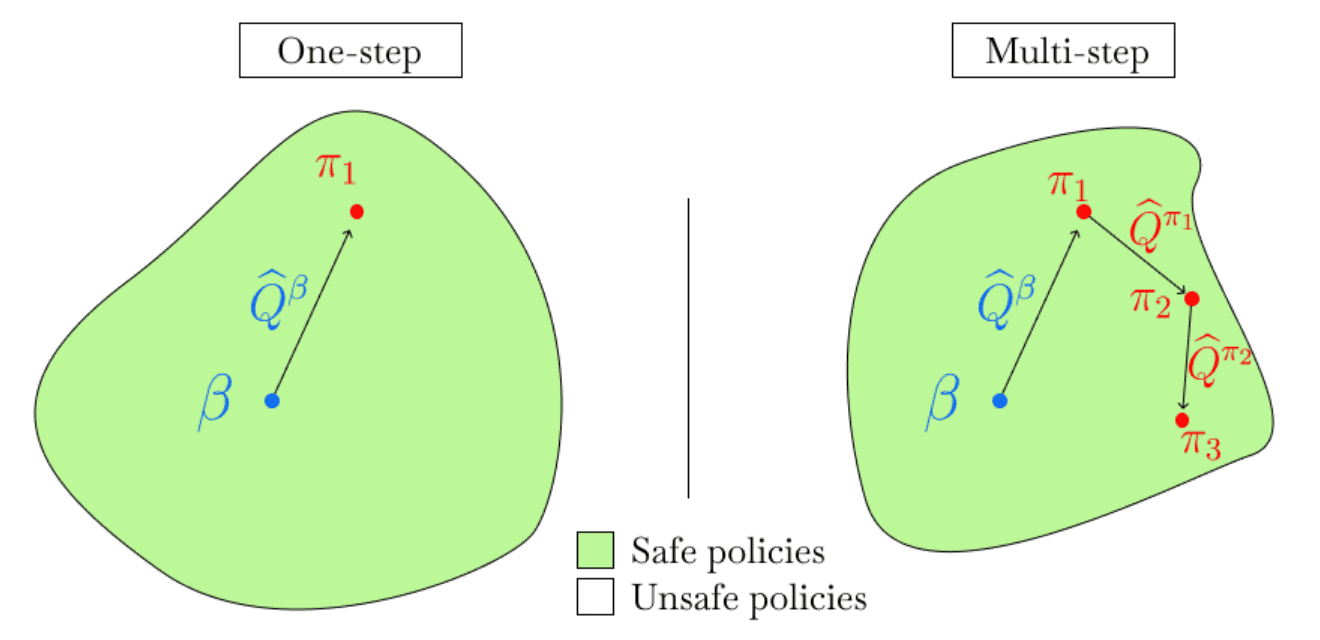
Many deep offline RL algorithms rely on an actor-critic framework, alternating between policy evaluation and policy improvement steps over multiple iterations (multi-step methods). Since the agent must use an off-policy $\pi_\theta$ distinct from the behavior policy $\pi_\beta$ after a single step of policy improvement, it is well-known that they are susceptible to the distribution shift problem.

To address the issue, explicit constraints such as regularization (e.g., SAC, CQL) or penalty terms (e.g., BCQ, TD3+BC) can be supplemented to restrict the agent policy $\pi_\theta$ to remain within the “safe” region around the behavior policy $\pi_\beta$. Nevertheless, querying or estimating values for unseen actions remains vulnerable to misestimation.

\[\texttt{General Offline RL: } \mathcal{L}(\theta) = \mathbb{E}_{(\mathbf{s}, \mathbf{a}, \mathbf{s}^\prime) \sim \mathcal{D}} \left[ \left( r (\mathbf{s}, \mathbf{a}) + \gamma \color{blue}{\max_{\mathbf{a}^\prime \in \mathcal{A}}} Q_{\hat{\theta}} (\mathbf{s}^\prime, \mathbf{a}^\prime) - Q_\theta (\mathbf{s}, \mathbf{a}) \right)^2 \right]\]

Instead, implicit Q-Learning (IQL) learns the optimal policy wihtout directly querying or estimating values for unseen actions, but with implicit constraints using advantage-weighted behavioral cloning.

\[\texttt{IQL: } \mathcal{L}(\theta) = \mathbb{E}_{(\mathbf{s}, \mathbf{a}, \mathbf{s}^\prime) \sim \mathcal{D}} \left[ \left( r (\mathbf{s}, \mathbf{a}) + \gamma \color{red}{\max_{\begin{gathered} \mathbf{a}^\prime \in \mathcal{A} \\ \text{ s.t. } \pi_\beta (\mathbf{a}^\prime \vert \mathbf{s}^\prime) > 0 \end{gathered}}} Q_{\hat{\theta}} (\mathbf{s}^\prime, \mathbf{a}^\prime) - Q_\theta (\mathbf{s}, \mathbf{a}) \right)^2 \right]\]

To do so, as we will see, IQL performs a single step of policy evaluation to learn an accurate estimate of $Q^{\pi_\beta} (\mathbf{s}, \mathbf{a})$, followed by a single-policy improvement step (one-step methods) to extract the best policy at once.

$\mathbf{Fig\ 1.}$ One-step v.s. Multi step methods (Brandfonbrener et al., 2021)

Preliminary: Expectile Regression

In the probability theory, the expectiles of a distribution are related to the expectation of the distribution in a way analogous to that in which the quantiles of the distribution are related to the median. Consider the random variable $X$ with the cdf $F$. Then, the expectation $\mathbb{E}[X]$ and the median $\mathrm{Med} (X)$ can be defined as the minimizer of the regression problem:

\[\begin{aligned} \mathbb{E}[X] & = \underset{m \in \mathbb{R}}{\arg \min} \; \mathbb{E} [(X - m)^2] \\ \mathrm{Med}(X) & = \underset{m \in \mathbb{R}}{\arg \min} \; \mathbb{E} \vert X - m \vert \end{aligned}\]

Analogously, $\tau$-quantile $q_\tau = F^{-1} (\tau)$ of $X$ can be defined as the minimizer of the following asymmetric $\mathcal{L}^1$ loss $\mathcal{L}_1^\tau (u) = \vert \tau - \mathbf{1}(u < 0) \vert \vert u \vert$:

\[\begin{aligned} q_\tau & = \underset{q \in \mathbb{R}}{\arg \min} \; \mathbb{E} [\mathcal{L}_1^\tau ( X - q )] \\ & = \underset{q \in \mathbb{R}}{\arg \min} \; \mathbb{E} \Bigl[ \vert X - q \vert \cdot (\tau \mathbf{1}(X > q) + (1 - \tau) \mathbf{1}(X < q)) \Bigr] \end{aligned}\]

And this problem is known as quantile regression. However, the non-smoothness of \(\mathcal{L}_1\) loss (thus not differentiable) complicates the optimization. Instead, a generalized quantity called the expectile $e_\tau$ is proposed as the minimizer of the following asymmetric $\mathcal{L}_2$ loss function $\mathcal{L}_2^\tau (u) = \vert \tau - \mathbf{1}(u < 0) \vert u^2$:

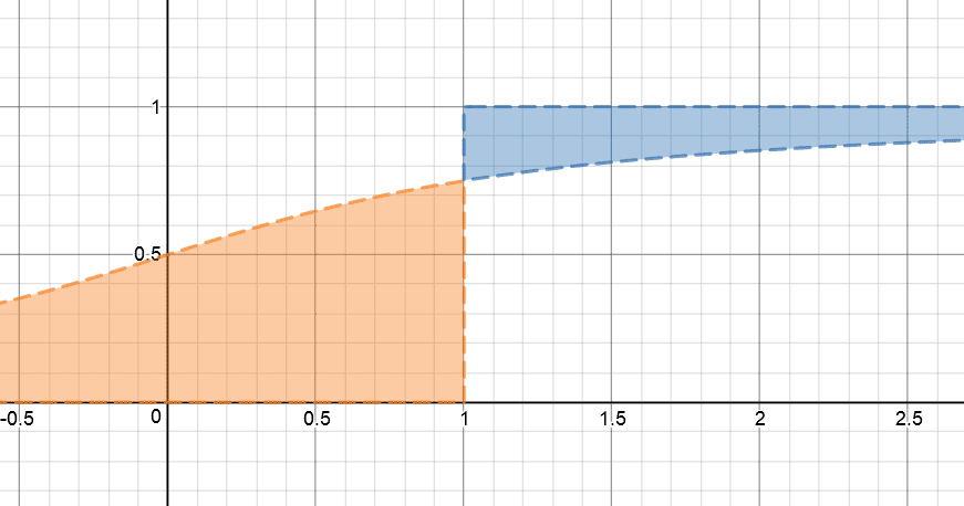
\[e_\tau = \underset{q \in \mathbb{R}}{\arg \min} \; \mathbb{E} [\mathcal{L}_2^\tau ( X - q )]\]

Intuitively, the expectile can be regarded as the quantile of the expectation as its name implies. In the visualization below, the dashed line represents the CDF of $X$. And the point $x = 1$ becomes the $q$-expectile if the proportion of the blue ($x > 1$) and orange ($x < 1$) area is equal to $(1−q)/q$.

\[\frac{\mathbb{E}[(X - e_\tau)_{+}]}{\mathbb{E}[(X - e_\tau)_{-}]} = \frac{1 - \tau}{\tau} \text{ where } x_+ = \max (x, 0) \text{ and } x_- = \min (x, 0)\]

$\mathbf{Fig\ 2.}$ Visualization of Expectile. (source: StackExchange)

Futhermore, it is mathematically known that expectile of $X$ is a quantile of a distribution distinct from $X$. For more mathematical interpretation, I recommend referring to Collin S. Philipps’ article.

Implicit Q-Learning

Q-Learning with Expectile Regression

TD-Learning (IQL)

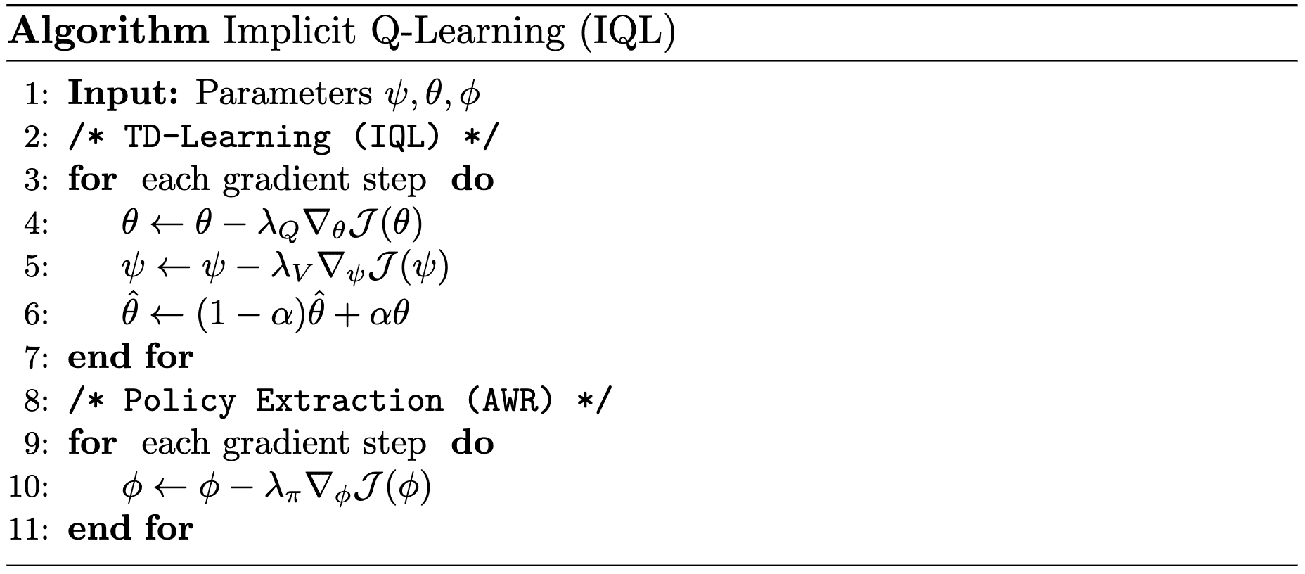
To avoid querying or estimating the values for unseen actions, implicit Q-learning leverages a function approximator $V_\psi$ for $V^\pi$ as the target, instead of using target actions sampled from $\mathbf{a}^* \sim \pi_\beta (\cdot \vert \mathbf{s}^\prime)$:

\[J(\theta) = \mathbb{E}_{(\mathbf{s}, \mathbf{a}, \mathbf{s}^\prime) \sim \mathcal{D}} [r (\mathbf{s}, \mathbf{a}) + V_\psi (\mathbf{s}^\prime) - Q_\theta (\mathbf{s}, \mathbf{a})]\]

To ensure the above update is meaningful, $V_\psi (\mathbf{s})$ should converge to $\max_{\mathbf{a} \in \mathcal{A}} Q_\theta (\mathbf{s}, \mathbf{a})$. Therefore, IQL also optimizes the following objective:

\[\mathcal{J} (\psi) = \mathbb{E}_{(\mathbf{s}, \mathbf{a}) \sim \mathcal{D}} [\mathcal{L} (Q_{\hat{\theta}} (\mathbf{s}, \mathbf{a}) - V_\psi (\mathbf{s}))]\]

for some loss metric $\mathcal{L} (\cdot)$ where $Q_\hat{\theta}$ is the target network, i.e., the EMA version of Q-network $Q_\theta$. For example, observe that the minimizer of the objective is \(V_\psi^* (\mathbf{s}) = \mathbb{E}_{\mathbf{a} \sim \pi_\beta (\cdot \vert \mathbf{s})} [Q_\theta (\mathbf{s}, \mathbf{a})]\) if $\mathcal{L}$ is set to MSE loss, aligning with the Bellman equations.

And the authors demonstrated that expectile regression (\(\mathcal{L}_2^\tau\) for $\mathcal{L}$) by setting larger values for $\tau$ allows us to satisfy the Bellman optimality equations, i.e., \(V_\psi^* (\mathbf{s}) = \max_{\mathbf{a} \in \mathcal{A}} Q_\theta (\mathbf{s}, \mathbf{a})\):

\[\begin{gathered} \mathcal{J} (\psi) = \mathbb{E}_{(\mathbf{s}, \mathbf{a}) \sim \mathcal{D}} [\mathcal{L}_2^\tau (Q_\hat{\theta} (\mathbf{s}, \mathbf{a} - V_\psi (\mathbf{s})))] \\ \text{ where } \mathcal{L}_2^\tau (u) = \vert \tau - \mathbf{1}(u < 0) \vert u^2 \end{gathered}\]

As we will see in the theoretical analysis, the minimizer $V_\tau$ of the above loss is the best value from the actions within the support of dataset $\mathcal{D}$:

\[\lim_{\tau \to 1} V_\tau (\mathbf{s}) = \max_{\begin{gathered} \mathbf{a} \in \mathcal{A} \\ \text{ s.t. } \pi_\beta (\mathbf{a} \vert \mathbf{s}) > 0 \end{gathered}} Q^* (\mathbf{s}, \mathbf{a})\]

Policy Extraction

After learning values by policy improvement steps, the policy $\pi_\phi$ is extracted using advantage weighted regression (AWR) with EMA version of Q-function $Q_\hat{\theta}$:

\[\mathcal{J} (\phi) = \mathbb{E}_{(\mathbf{s}, \mathbf{a}) \sim \mathcal{D}}[ \exp \left( \beta ( Q_{\hat{\theta}}(\mathbf{s}, \mathbf{a}) - V_\psi (\mathbf{s})) \right) \log \pi_\phi (\mathbf{a} \vert \mathbf{s})]\]

where $\beta \in [0, \infty)$ is an inverse temperature.

Algorithm

$\mathbf{Fig\ 3.}$ The pseudocode for Implicit Q-Learning

Theoretical Analysis

Let $V^\tau (\mathbf{s})$ be the optimal solution of minimizing $\mathcal{L}(\psi)$, i.e. $\tau$-expectile of $Q_\theta (\mathbf{s}, \mathbf{a})$ and $Q^\tau$ be the optimal solution for $L (\theta)$. That is, recursively:

\[\begin{aligned} V_\tau (\mathbf{s}) & = \mathbb{E}_{\mathbf{a} \sim \pi_\beta (\cdot \vert \mathbf{s})}^\tau [Q_\tau (\mathbf{s}, \mathbf{a})] \\ Q_\tau (\mathbf{s}, \mathbf{a}) & = r(\mathbf{s}, \mathbf{a}) + \gamma \mathbb{E}_{\mathbf{s}^\prime \sim \mathbb{P}(\cdot \vert \mathbf{s}, \mathbf{a})} [V_\tau (\mathbf{s}^\prime)] \end{aligned}\]

where $\mathbb{E}_{x \sim X}^\tau [x]$ denotes the $\tau$-expectile of $X$. To prove the main convergence theorem, we require the following lemmas:

$\color{green}{\mathbf{Lemma.}}$ Let $X$ be a real-valued random variable with a bounded support, and $x^*$ be the supremum of the support. Then, for $\tau$-expectile $e_\tau$ of $X$: $$ \lim_{\tau \to 1} e_\tau = x^* $$

$\mathbf{Proof.}$

Note that expectiles of a random variable have the same supremum $x^*$.

Moreover, for all $\tau_1 < \tau_2$, it is obvious that $e_{\tau_1} \leq e_{\tau_2}$ from the fact that the expectile can be regarded as the quantile of another distribution.

Therefore, the convergence and its limit follow from the monotone convergence theorem.

\[\tag*{$\blacksquare$}\]

$\color{green}{\mathbf{Lemma.}}$ Monotonicity
For any state $\mathbf{s} \in \mathcal{S}$ and $\tau_1 < \tau_2$, we have: $$ V_{\tau_1} (\mathbf{s}) \leq V_{\tau_2} (\mathbf{s}) $$

$\mathbf{Proof.}$

The proof is equals to the general policy improvement proof:

\[\begin{aligned} & V_{\tau_1}(\mathbf{s}) = \mathbb{E}_{\mathbf{a} \sim \pi_\beta (\cdot \vert \mathbf{s})}^{\tau_1} \left[r(\mathbf{s}, \mathbf{a}) + \gamma \mathbb{E}_{\mathbf{s}^\prime \sim \mathbb{P}(\cdot \vert \mathbf{s}, \mathbf{a})} \left[ V_{\tau_1} (\mathbf{s}^{\prime}) \right] \right] \\ & \leq \mathbb{E}_{\mathbf{a} \sim \pi_\beta (\cdot \vert \mathbf{s})}^{\tau_2} \left[ r(\mathbf{s}, \mathbf{a}) + \gamma \mathbb{E}_{\mathbf{s}^\prime \sim \mathbb{P}(\cdot \vert \mathbf{s}, \mathbf{a})} \left[ V_{\tau_1} (\mathbf{s}^\prime) \right] \right] \\ & = \mathbb{E}_{\mathbf{a} \sim \pi_\beta (\cdot \vert \mathbf{s})}^{\tau_2}\left[r(\mathbf{s}, \mathbf{a}) + \gamma \mathbb{E}_{\mathbf{s}^\prime \sim \mathbb{P}(\cdot \vert \mathbf{s}, \mathbf{a})} \mathbb{E}_{\mathbf{a}^\prime \sim \pi_\beta (\cdot \vert \mathbf{s}^\prime)}^{\tau_1} \left[r(\mathbf{s}^\prime, \mathbf{a}^\prime) + \gamma \mathbb{E}_{\mathbf{s}^{\prime \prime} \sim \mathbb{P}(\cdot \vert \mathbf{s}^\prime, \mathbf{a}^\prime)}\left[V_{\tau_1}\left(\mathbf{s}^{\prime \prime}\right)\right]\right]\right] \\ & \leq \mathbb{E}_{\mathbf{a} \sim \pi_\beta (\cdot \vert \mathbf{s})}^{\tau_2}\left[r(\mathbf{s}, \mathbf{a})+\gamma \mathbb{E}_{\mathbf{s}^\prime \sim \mathbb{P}(\cdot \vert \mathbf{s}, \mathbf{a})} \mathbb{E}_{\mathbf{a}^\prime \sim \pi_\beta \left(\cdot \vert \mathbf{s}^\prime\right)}^{\tau_2}\left[r\left(\mathbf{s}^\prime, \mathbf{a}^\prime\right)+\gamma \mathbb{E}_{\mathbf{s}^{\prime \prime} \sim \mathbb{P}(\cdot \vert \mathbf{s}^\prime, \mathbf{a}^\prime)}\left[V_{\tau_1}\left(\mathbf{s}^{\prime \prime}\right)\right]\right]\right] \\ & =\mathbb{E}_{\mathbf{a} \sim \pi_\beta (\cdot \vert \mathbf{s})}^{\tau_2}\left[r(\mathbf{s}, \mathbf{a})+\gamma \mathbb{E}_{\mathbf{s}^\prime \sim \mathbb{P}(\cdot \vert \mathbf{s}, \mathbf{a})} \mathbb{E}_{\mathbf{a}^\prime \sim \pi_\beta \left(\cdot \vert \mathbf{s}^\prime\right)}^{\tau_2}\left[r\left(\mathbf{s}^\prime, \mathbf{a}^\prime\right)+\gamma \mathbb{E}_{\mathbf{s}^{\prime \prime} \sim \mathbb{P}(\cdot \vert \mathbf{s}^\prime, \mathbf{a}^\prime)} \mathbb{E}_{a^{\prime \prime} \sim \pi_\beta \left(\cdot \vert \mathbf{s}^{\prime \prime}\right)}^{\tau_1}\left[r\left(\mathbf{s}^{\prime \prime}, a^{\prime \prime}\right)+\ldots\right]\right]\right] \\ & \vdots \\ & \leq V_{\tau_2}(s) \\ \end{aligned}\] \[\tag*{$\blacksquare$}\]

By the previous lemma, the following corollary holds:

$\color{blue}{\mathbf{Corollary.}}$ Boundedness
For any $\tau \in (0, 1)$ and $\mathbf{s} \in \mathcal{S}$, we have: $$ V_\tau (\mathbf{s}) \leq \max_{\begin{gathered} \mathbf{a} \in \mathcal{A} \\ \text{ s.t. } \pi_\beta (\mathbf{a} \vert \mathbf{s}) > 0 \end{gathered}} Q^* (\mathbf{s}, \mathbf{a}) $$ where $Q^* (\mathbf{s}, \mathbf{a})$ is an optimal state-action value function constrained to the dataset and defined as: $$ Q^* (\mathbf{s}, \mathbf{a}) = r(\mathbf{s}, \mathbf{a}) + \gamma \mathbb{E}_{\mathbf{s}^\prime \sim \mathbb{P}(\cdot \vert \mathbf{s}, \mathbf{a})} \left[ \max_{\begin{gathered} \mathbf{a}^\prime \in \mathcal{A} \\ \text{ s.t. } \pi_\beta (\mathbf{a}^\prime \vert \mathbf{s}^\prime) > 0 \end{gathered}} Q^* (\mathbf{s}^\prime, \mathbf{a}^\prime) \right] $$

$\mathbf{Proof.}$

By prior lemmas, $V_\tau$ for any $\tau$ is upper-bounded by the supremum of $Q_\theta (\mathbf{s}, \mathbf{a})$ in the support of $\pi_\beta$. Note that convex combination is smaller than maximum:

\[\sum_{i=1}^n a_i z_i \leq \max_{i \in \{1, \cdots, n\}} z_i \quad \text{ where } \sum_{i=1}^n a_i = 1\]

By this mathematical fact and definitions of value functions and optimal value functions, the supremum of $Q_\theta (\mathbf{s}, \mathbf{a})$ in the support of $\pi_\beta$ is trivially

\[\max_{\begin{gathered} \mathbf{a} \in \mathcal{A} \\ \text{ s.t. } \pi_\beta (\mathbf{a} \vert \mathbf{s}) > 0 \end{gathered}} Q^* (\mathbf{s}, \mathbf{a})\] \[\tag*{$\blacksquare$}\]

Therefore, by monotone convergence theorem, the main theorem is now trivial:

$\color{red}{\mathbf{Theorem.}}$ Convergence of Value Target
$$ \lim_{\tau \to 1} V_\tau (\mathbf{s}) = \max_{\begin{gathered} \mathbf{a} \in \mathcal{A} \\ \text{ s.t. } \pi_\beta (\mathbf{a} \vert \mathbf{s}) > 0 \end{gathered}} Q^* (\mathbf{s}, \mathbf{a}) $$

$\mathbf{Proof.}$

Done by the monotone convergence theorem, combining lemmas and the collorary.

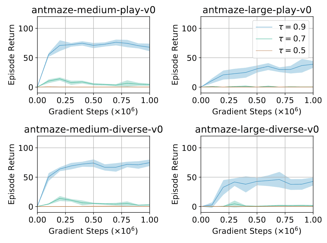
\[\tag*{$\blacksquare$}\]

And this theorem aligns with the authors’ experimental observations that estimating a larger expectile $\tau$ is crucial for antmaze tasks that require dynamical programming to combine parts of suboptimal trajectories.

$\mathbf{Fig\ 4.}$ Effectiveness of larger expectile $\tau$ (Kostrikov et al., 2022)

Importance of Value Target

From the theoretical analysis, the straightforward approach to approximates the maximum of TD target $r(\mathbf{s}, \mathbf{a}) + \gamma \max_{\mathbf{a}^\prime \in \mathcal{A}} Q_\hat{\theta} (\mathbf{s}^\prime, \mathbf{a}^\prime)$ is simply the following expectile regression objective:

\[\mathcal{L}^\prime (\theta) = \mathbb{E}_{(\mathbf{s}, \mathbf{a}, \mathbf{s}^\prime, \mathbf{a}^\prime) \sim \mathcal{D}} [ \mathcal{L}_2^\tau \left( r (\mathbf{s}, \mathbf{a}) + \gamma Q_\hat{\theta} (\mathbf{s}^\prime, \mathbf{a}^\prime) - Q_\theta (\mathbf{s}, \mathbf{a}) \right)]\]

However, it’s important to learn a value function since otherwise maximization will be performed not only over $\mathbf{a}^\prime$ but also over $\mathbf{s}^\prime \sim \mathbb{P}(\cdot \vert \mathbf{s}, \mathbf{a})$. Specifically, a large target value might not necessarily indicate the existence of a single action that achieves that value, but rather a “lucky” sample that happened to transition into a good state.

Experimental Results

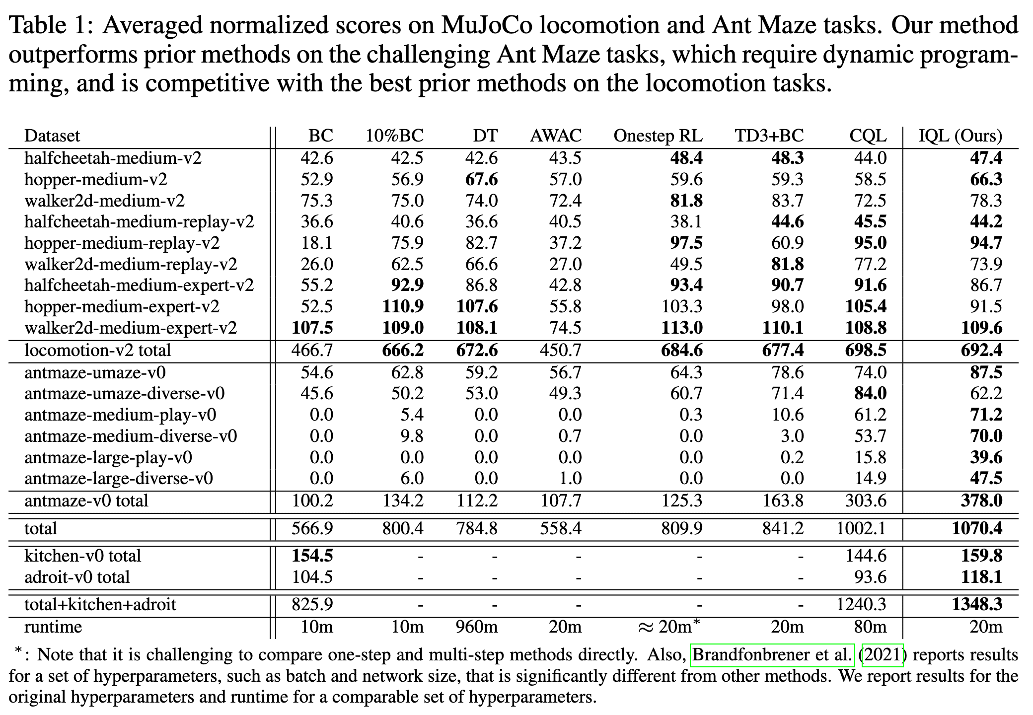
Although prior one-step methods (Brandfonbrener et al., 2021) perform very poorly on more complex datasets in D4RL, which require combining parts of suboptimal trajectories, IQL can correctly find near-optimal policies in such scenarios.

The key difference between IQL and the one-step methods proposed byBrandfonbrener et al., 2021 is that IQL performs iterative dynamic programming for the value updates, which are based on the Bellman optimality equation. Therefore, IQL offers an appealing combination of the strengths of both one-step and multi-step methods.

$\mathbf{Fig\ 5.}$ Brandfonbrener et al., 2021 v.s. IQL on toy umaze environment (Kostrikov et al., 2022)

Consequently, IQL has demonstrated to be one of the most successful methods on the D4RL benchmark, exhibiting robust and consistent performance across multiple domains with varying complexity, from AntMaze to Adroit.

$\mathbf{Fig\ 6.}$ Comparisons of offline RL algorithms (Kostrikov et al., 2022)

References

[1] Kostrikov et al., “Offline Reinforcement Learning with Implicit Q-Learning”, ICLR 2022 Poster
[2] Brandfonbrener et al., “Offline RL Without Off-Policy Evaluation”, NeurIPS 2021
[3] Wikipedia, Quantile regression
[4] Collin S. Philipps, Interpreting Expectiles