[RL] Offline Model-Based RL
Direct application of MBRL algorithms to offline settings can be problematic due to the distribution shifts and the inability of offline-learned models to correct errors through environmental interaction. Since the offline dataset may not cover the entire state-action space, the learned models are unlikely to be globally accurate. Consequently, planning with the learned model without any safeguards against model inaccuracy can result in model exploitation, yielding poor results. In this post, we explore some previous efforts to adapt MBRL for offline setting.
MOReL: Model-based Offline RL
Kidambi et al., 2020 proposed a method named model-based offline RL (MOReL) that consists of two modular steps:
- Learning pessimistic MDP (P-MDP) with the offline dataset
The P-MDP partitions the state space into "known" and "unknown" regions, and uses a large negative reward for unknown regions. This provides a regularizing effect during policy learning by heavily penalizing policies that visit unknown states. In contrast, model-free algorithms are forced to regularize the policies directly towards the data logging policy, which can be overly conservative. - Learning near-optimal policy for the P-MDP
For any policy, the performance in the true MDP (real environment) is approximately lower-bounded by the performance in the P-MDP. making it a suitable surrogate for purposes of policy evaluation and learning, and overcome common pitfalls of model-based RL like model exploitation.

Pessimistic MDP (P-MDP)
To partition the state-action space into known and unknown regions, they proposed a measure of disagreement between the true dynamics and learned model:
Let $\hat{\mathbb{P}}(\cdot \vert \mathbf{s}, \mathbf{a})$ be an approximate dynamics model of the true dynamics $\mathbb{P}(\cdot \vert \mathbf{s}, \mathbf{a})$. Given a state-action pair $(\mathbf{s}, \mathbf{a})$, define an unknown state action detector as: $$ U^\alpha (\mathbf{s}, \mathbf{a}) = \begin{cases} \textrm{FALSE (i.e. Known)} & \mathrm{if} \quad \mathrm{TV} \left( \hat{\mathbb{P}}(\cdot \vert \mathbf{s}, \mathbf{a}), \mathbb{P}(\cdot \vert \mathbf{s}, \mathbf{a}) \right) \leq \alpha \text{ can be guaranteed} \\ \textrm{TRUE (i.e. Unknown)} & \mathrm{otherwise} \end{cases} $$
Then, a pessimistic MDP (P-MDP) can be constructed using the learned model and USAD by penalizing policies that venture into unknown parts of state-action space:
The $(\alpha, \kappa)$-pessimistic MDP $\hat{\mathcal{M}}_p$ is described by a set of tuples: $$ \hat{\mathcal{M}}_p := \{ S \cup \texttt{HALT}, A, r_p, \hat{\mathbb{P}}_p, \hat{\rho}_0, \gamma \} $$
- $(S, A)$ are states and actions in the true MDP (environment) $\mathcal{M}$.
- $\texttt{HALT}$ is an additional absorbing state.
- $\hat{\rho}_0$ is the initial state distribution learned from the dataset $\mathcal{D}$.
- $\gamma$ is the discount factor (same as $\mathcal{M}$).
- The modified reward and transition dynamics are given by: $$ \begin{split} \hat{\mathbb{P}}_{p}(\mathbf{s}^\prime \vert \mathbf{s}, \mathbf{a}) = \begin{cases} \delta(\mathbf{s}^\prime=\texttt{HALT}) & \begin{array}{l} \mathrm{if} \; U^\alpha(\mathbf{s}, \mathbf{a}) = \mathrm{TRUE} \\ \mathrm{or} \; \mathbf{s} = \texttt{HALT} \end{array} \\ \hat{\mathbb{P}}(\mathbf{s}^\prime \vert \mathbf{s}, \mathbf{a}) & \mathrm{otherwise} \end{cases} \end{split} \quad \begin{split} r_p (\mathbf{s}, \mathbf{a}) = \begin{cases} -\kappa & \mathrm{if} \; \mathbf{s} = \texttt{HALT} \\ r(\mathbf{s}, \mathbf{a}) & \mathrm{otherwise} \end{cases} \end{split} $$ That is, the P-MDP forces the original MDP to transition to the absorbing state $\texttt{HALT}$ for unknown state-action pairs. And unknown state-action pairs are penalized by a negative reward of $−\kappa$, while all known state-actions receive the same reward as in the environment.
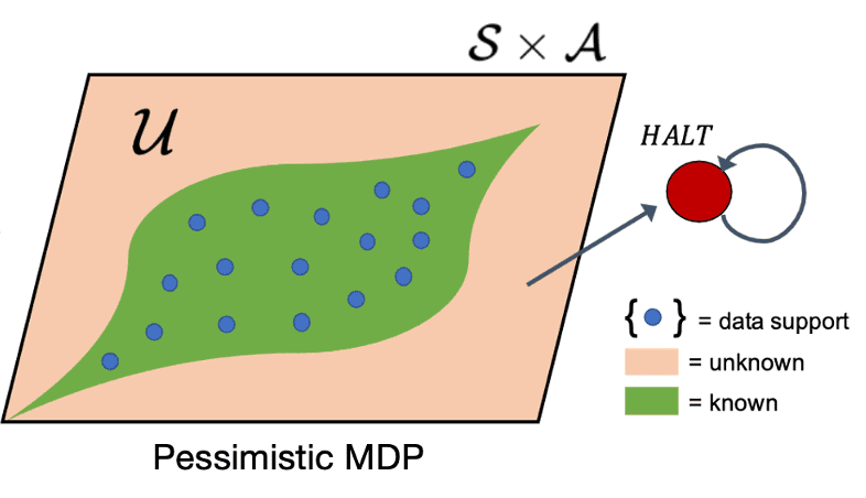
In the practical implementation, the uncertainty distance of USAD (i.e., TV distance) is approximated by the predictions of ensembles of models \(\{ f_{\phi_1}, f_{\phi_2}, \cdots \}\) where each model uses a different weight initialization and are optimized with different mini-batch sequences:
\[\texttt{disc} (\mathbf{s}, \mathbf{a}) = \max_{i, j} \Vert f_{\phi_i} (\mathbf{s}, \mathbf{a}) - f_{\phi_j} (\mathbf{s}, \mathbf{a}) \Vert_2\]That is, the practical $\alpha$-USAD is given by:
\[U_{\texttt{practical}}^\alpha (\mathbf{s}, \mathbf{a}) = \begin{cases} \textrm{FALSE (i.e. Known)} & \mathrm{if} \quad \texttt{disc} (\mathbf{s}, \mathbf{a}) \leq \mathrm{threshold} \\ \textrm{TRUE (i.e. Unknown)} & \mathrm{otherwise} \end{cases}\]Pessimistic Policy Learning
After defining P-MDP, the final step in MOReL is to perform planning within the P-MDP that provides a good safeguards against the inaccurate and unknown regions of the learned model, which may cause distribution shift and model exploitation, extracting the final policy $\pi_{\texttt{out}}$.

Although the P-MDP is pessimistic in the sense that it only offers validated $(\mathbf{s}, \mathbf{a})$ pairs to the agent, the authors demonstrated that it serves as a suitable approximation of the MDP, thereby effectively transferring its learning progress to the actual environment. For theoretical analysis, first define the notion of hitting time to denote the moment when the agents first enter the unknown regions:
Given an MDP $\mathcal{M}$, starting state distribution $\rho_0$, state-action pair $(\mathbf{s}, \mathbf{a})$, and policy $\pi$, the hitting time $\mathcal{T}_{(\mathbf{s}, \mathbf{a})}$^\pi is defined as the random variable denoting the first time action $\mathbf{a}$ is taken at state $\mathbf{s}$ by $\pi$ on $\mathcal{M}$. $$ \mathcal{T}_{(\mathbf{s}, \mathbf{a})}^\pi = \min_{t \in \mathbb{N}} \left( t \cdot \delta (\mathbf{s}_t = \mathbf{s}, \mathbf{a}_t = \mathbf{a}) \right) $$ It is equal to $\infty$ if $\mathbf{a}$ is never taken by $\pi$ from state $\mathbf{s}$. For a set of state-action pairs $V \subseteq \mathcal{S} \times \mathcal{A}$, we also define $$ \mathcal{T}_V^\pi = \min_{(\mathbf{s}, \mathbf{a}) \in V} \mathcal{T}_{(\mathbf{s}, \mathbf{a})}^\pi $$
And let’s denote expected performance on the environment $\mathcal{M}$ with states sampled according to $\rho_0$ as:
\[\mathcal{J}_{\rho_0} (\pi, \mathcal{M}) = \mathbb{E}_{\mathbf{s} \sim \rho_0} [V_\pi (\mathbf{s}, \mathcal{M})] \text{ where } V_\pi (\mathbf{s}, \mathcal{M}) = \mathbb{E} \left[ \sum_{t=0}^\infty \gamma^t r(\mathbf{s}_t, \mathbf{a}_t) \middle\vert \mathbf{s}_0 = \mathbf{s} \right]\]The following main theorem suggests that the value of a policy in the P-MDP cannot substantially exceed the value in the environment. This makes the value in the P-MDP an approximate lower-bound on the true performance, and a good surrogate for optimization.
The value of any policy $\pi$ on the original MDP $\mathcal{M}$ and its $(\alpha, R_{\max})$-pessimistic MDP $\hat{\mathcal{M}}_p$ satisfies: $$ \begin{aligned} \mathcal{J}_{\hat{\rho}_0}(\pi, \hat{\mathcal{M}}_p) &\geq \mathcal{J}_{\rho_0}(\pi, \mathcal{M}) - \frac{2 R_{\max}}{1-\gamma} \cdot \mathrm{TV}(\rho_0, \hat{\rho}_0) - \frac{2 \gamma R_{\max}}{(1-\gamma)^2} \cdot \alpha - \frac{2 R_{\max}}{1-\gamma} \cdot \mathbb{E}\left[\gamma^{\mathcal{T}_\mathcal{U}^\pi}\right] \\ \mathcal{J}_{\hat{\rho}_0}(\pi, \hat{\mathcal{M}}_p) &\leq \mathcal{J}_{\rho_0}(\pi, \mathcal{M}) + \frac{2 R_{\max}}{1-\gamma} \cdot \mathrm{TV}(\rho_0, \hat{\rho}_0) + \frac{2 \gamma R_{\max}}{(1-\gamma)^2}\cdot \alpha \end{aligned} $$ where $\mathcal{T}_\mathcal{U}^\pi$ denotes the hitting time of unknown states by $\pi$ on $\mathcal{M}$: $$ \mathcal{U} = \{ (\mathbf{s}, \mathbf{a}) \vert U^\alpha (\mathbf{s}, \mathbf{a}) = \mathrm{TRUE} \} $$
$\mathbf{Proof.}$
To prove the theorem, define another P-MDP $\mathcal{M}_p$, which is the same as $\hat{\mathcal{M}}_p$ except that the intial state distribution is $\rho_0$ instead of $\hat{\rho}_0$ and the transition probability from a known state-action pair $(\mathbf{s}, \mathbf{a})$ is $\mathbb{P}(\mathbf{s}^\prime \vert \mathbf{s}, \mathbf{a})$ instead of learned $\hat{\mathbb{P}} (\mathbf{s}^\prime \vert \mathbf{s}, \mathbf{a})$.
The main idea of the overall proof of the claims below is to couple the evolutions of any given policy on the pessimistic MDP $\mathcal{M}_p$ and the model-based pessimistic MDP $\hat{\mathcal{M}}_p$:
$\mathbf{Proof.}$
Suppose that such a coupling can be performed in the first step. Since \(\Vert \mathbb{P}(\cdot \vert \mathbf{s}, \mathbf{a}) - \hat{\mathbb{P}}(\cdot \vert \mathbf{s}, \mathbf{a}) \Vert_1 \leq \alpha\) for known $(\mathbf{s}, \mathbf{a})$, this coupling can be performed at each subsequent step with probability $1 − \alpha$. With similar arguments, the probability that the coupling is not valid at time $t$ is at most $1 − (1 − \alpha)^t$. Therefore:
\[\begin{align*} \Bigl\vert \mathcal{J}_{\hat{\rho}_0}(\pi, \hat{\mathcal{M}}_p) - \mathcal{J}_{\rho_0}(\pi,\mathcal{M}_p) \Bigr\vert & \leq \frac{2 R_{\max}}{1-\gamma} \cdot \mathrm{TV}(\rho_0, \hat{\rho}_0) + \sum_t \gamma^t \left( 1 - (1-\alpha)^t \right) \cdot 2\cdot R_{\max} \\ &\leq \frac{2R_{\max}}{1-\gamma} \cdot \mathrm{TV}(\rho_0, \hat{\rho}_0) + \frac{2 \gamma R_{\max}}{(1-\gamma)^2} \cdot \alpha. \end{align*}\] \[\tag*{$\blacksquare$}\]Now, by the following claim, the main theorem is proved.
$\mathbf{Proof.}$
For the first inequality, observe that the evolution of any policy $\pi$ on the pessimistic MDP $\mathcal{M}p$, can be coupled with the evolution of π on the actual MDP $\mathcal{M}$ until $\pi$ encounters an unknown state. From this point, the total rewards obtained on the pessimistic MDP $\mathcal{M}_p$ will be $\frac{-R{\max}}{1-\gamma}$, while the maximum total reward obtained by $\pi$ on $\mathcal{M}$ from that point on is $\frac{-R_{\max}}{1 -\gamma}$. By multiplying by the discount factor \(\mathbb{E} \left[ \gamma^{ \mathcal{T}_\mathcal{U}^\pi}\right]\), done.
For the second inequality, consider any policy $\pi$ and let it evolve on the MDP $\mathcal{M}$ as $(\mathbf{s}, \mathbf{a}, \mathbf{s}\mathcal{M}^\prime)$. Simulate an evolution of the same policy $\pi$ on $\mathcal{M}_p$, $\left(\mathbf{s}, \mathbf{a}, \mathbf{s}{\mathcal{M}_p}^\prime \right)$ as follows:
- If $(\mathbf{s}, \mathbf{a}) \in \mathcal{U}$, then $\mathbf{s}_{\mathcal{M}_p}^\prime = \texttt{HALT}$
- Otherwise, $\mathbf{s}_{\mathcal{M}_p}^\prime = \mathbf{s}_{\mathcal{M}}^\prime$
Observe that the rewards obtained by π on each transition in $\mathcal{M}_p$ is less than or equal to that obtained by $\pi$ on the same transition in $\mathcal{M}$.
\[\tag*{$\blacksquare$}\]Note that this theorem also bound the suboptimality of output policy $\pi_{\texttt{out}}$:
Suppose the PLANNER of MOReL returns an $\varepsilon_\pi$ sub-optimal policy. Then, we obtain: $$ \mathcal{J}_{\rho_0}(\pi^*, \mathcal{M}) - \mathcal{J}_{\rho_0}(\pi_{\texttt{out}}, \mathcal{M}) \leq \varepsilon_{\pi} + \frac{4 R_{\max}}{1-\gamma} \cdot \mathrm{TV}(\rho_0, \hat{\rho}_0) + \frac{4\gamma R_{\max}}{(1-\gamma)^2} \cdot \alpha + \frac{2 R_{\max}}{1-\gamma} \cdot \mathbb{E} \left[ \gamma^{\mathcal{T}_{\mathcal{U}}^{\pi^*}} \right]. $$
Empirical Results
MOReL achieves the highest normalized score in 5 out of 12 domains of D4RL, whereas the next best algorithm (CQL) achieves the highest score in only 3 out of 12 domains. Furthermore, the authors observed that MOReL is often highly competitive with the best-performing algorithm in any given domain, even when it doesn’t achieve the top score.
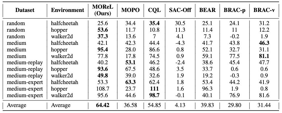
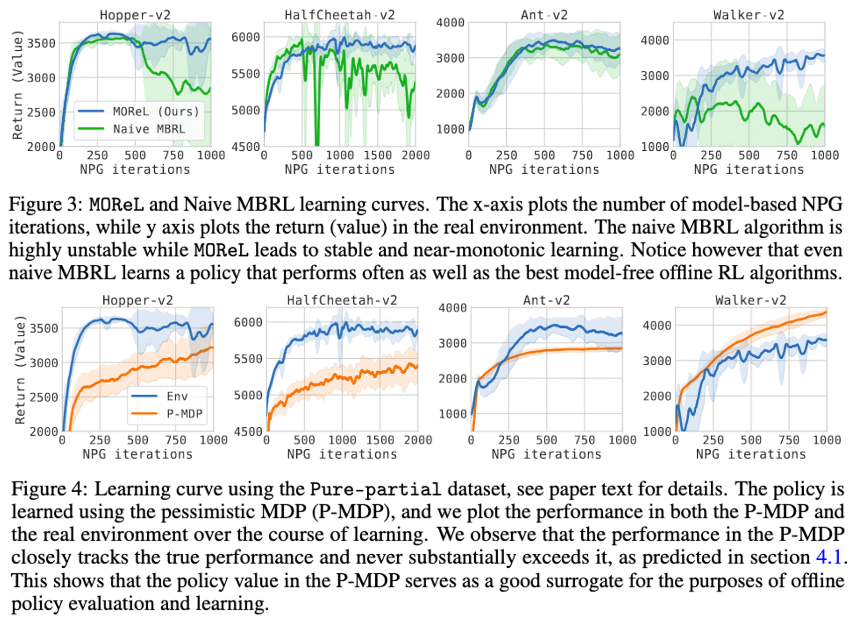
Furthermore, the authors empirically demonstrated the theoretical properties of P-MDP:
- While the learned model is being over-exploited, the learning curve of MOReL remains stable and nearly monotonic, even after various steps of policy improvement.
- The value in the true environment closely correlates with the value in P-MDP. Notably, the P-MDP value never significantly exceeds the true performance, suggesting that the pessimism helps to prevent model exploitation.
MOPO: Model-based Offline Policy Optimization
Similar to MOReL, model-based offline policy optimization (MOPO) by Yu et al., 2020 also optimizes a policy in an uncertainty-penalized MDP, where the reward function is penalized by an estimate $u (\mathbf{s}, \mathbf{a})$ of the model’s error. This safe MDP theoretically enables the agent to maximize a lower bound of the return in the true MDP.
Unlike MOReL, which constructs terminating states $\texttt{HALT}$ based on a hard threshold on uncertainty, MOPO uses a soft reward penalty to incorporate uncertainty. Specifically, MOPO quantifies the uncertainty as the maximum $\Vert \cdot \Vert_F$ among the ensemble of multivariate Gaussian dynamic models \(\hat{\mathbb{P}}_{\theta, \phi}^i (\mathbf{s}^\prime \vert \mathbf{s}, \mathbf{a}) = \mathcal{N}(\mu_\theta^i (\mathbf{s}, \mathbf{a}), \Sigma_\phi^i (\mathbf{s}, \mathbf{a}))\):
\[\begin{aligned} & \texttt{MOReL: } \tilde{r}(\mathbf{s}, \mathbf{a}) = \begin{cases} r(\mathbf{s}, \mathbf{a}) & \mathrm{if} \; \max_{i, j} \Vert f_{\phi_i} (\mathbf{s}, \mathbf{a}) - f_{\phi_j} (\mathbf{s}, \mathbf{a}) \Vert_2 \leq \alpha \\ - R_{\max} & \mathrm{otherwise} \end{cases} \\ & \\ & \texttt{MOPO: } \tilde{r}(\mathbf{s}, \mathbf{a}) = r (\mathbf{s}, \mathbf{a}) - \lambda \max_{1 \leq i \leq N} \Vert \Sigma_\phi^i (\mathbf{s}, \mathbf{a}) \Vert_F \end{aligned}\]Uncertainty-Penalized MDPs
Given an error estimator $u (\mathbf{s}, \mathbf{a})$, the uncertainty-penalized MDP is defined as follows:
The uncertainty-penalized MDP $\widetilde{\mathcal{M}}$ is defined by tuple $(\mathcal{S}, \mathcal{A}, \hat{\mathbb{P}}, \tilde{r}, \mu_0, \gamma)$ where $\hat{\mathbb{P}}$ is the learned dynamics and $\tilde{r}$ is the uncertainty-penalized reward: $$ \tilde{r} (\mathbf{s}, \mathbf{a}) := r(\mathbf{s}, \mathbf{a}) - \lambda u (\mathbf{s}, \mathbf{a}) $$
The following theorem shows that the return on $\widetilde{\mathcal{M}}$ lower-bounds the true return of the real environment $\mathcal{M}$:
Let $d_\mathcal{F}$ be an integral probability metric (IPM) defined by a function class $\mathcal{F}$ and denote the true value function as $V_\mathcal{M}^\pi$: $$ V_\mathcal{M}^\pi (\mathbf{s}) = \mathbb{E}_{\pi, \mathbb{P}} \left[ \sum_{t=0}^\infty \gamma^t r (\mathbf{s}_t, \mathbf{a}_t) \middle\vert \mathbf{s}_0 = \mathbf{s} \right] $$ Assume that:
- We can represent the value function with $\mathcal{F}$
For any policy $\pi$, $V_\mathcal{M}^\pi \in c \mathcal{F}$ for some scalar $c \in \mathbb{R}$. - The model error is bounded above by $u (\mathbf{s}, \mathbf{a})$
$u$ is an admissible estimator for learned dynamics $\hat{\mathbb{P}}$ in the sense that: $$ \forall (\mathbf{s}, \mathbf{a}) \in \mathcal{S} \times \mathcal{A}: \quad d_\mathcal{F} (\hat{\mathbb{P}} (\cdot \vert \mathbf{s}, \mathbf{a}), \mathbb{P} (\cdot \vert \mathbf{s}, \mathbf{a})) \leq u(\mathbf{s}, \mathbf{a}) $$
$\mathbf{Proof.}$
One of the natural way to quantify the uncertainty of learned MDP $\hat{\mathcal{M}}$ on $(\mathbf{s}, \mathbf{a})$ is to compare the performance of a policy under true MDP $\mathcal{M}$. Firstly, for the value function $V_\mathcal{M}^\pi$ of policy $\pi$ on MDP $\mathcal{M}$, we can quantify the uncertainty on a single state-action $(\mathbf{s}, \mathbf{a})$ by comparing future return of two MDPs:
\[G_{\hat{\mathcal{M}}}^\pi (\mathbf{s}, \mathbf{a}) = \mathbb{E}_{\mathbf{s}^\prime \sim \hat{\mathbb{P}}(\cdot \vert \mathbf{s}, \mathbf{a})} [V_\hat{\mathcal{M}}^\pi (\mathbf{s}^\prime)] - \mathbb{E}_{\mathbf{s}^\prime \sim \mathbb{P}(\cdot \vert \mathbf{s}, \mathbf{a})} [V_\mathcal{M}^\pi (\mathbf{s}^\prime)]\]Then, we can represent the difference of overall performance of $\pi$ between two MDPs with $G_{\hat{\mathcal{M}}}^\pi$, using the following telescoping lemma:
Let $P_{\hat{\mathbb{P}}, t}^\pi (\mathbf{s})$ denote the probability of being in state $\mathbf{s}$ at time step $t$ if actions are sampled according to $\pi$ and transitions according to $\hat{\mathbb{P}}$, and $\rho_{\hat{\mathbb{P}}}^\pi (\mathbf{s}, \mathbf{a})$ be the discounted occupancy measure of policy $\pi$ under dynamics $\hat{\mathbb{P}}$: $$ \rho_{\hat{\mathbb{P}}}^\pi (\mathbf{s}, \mathbf{a}) = \pi (\mathbf{a} \vert \mathbf{s}) \sum_{t = 0}^\infty \gamma^t P_{\hat{\mathbb{P}}, t}^\pi (\mathbf{s}) $$ That is, the performance of $\pi$ is given by $\mathcal{J} (\pi, \hat{\mathcal{M}}) = \mathbb{E}_{\rho_{\hat{\mathbb{P}}}^\pi} [r(\mathbf{s}, \mathbf{a})]$. Then we have: $$ \mathcal{J} (\pi, \hat{\mathcal{M}}) - \mathcal{J} (\pi, \mathcal{M}) = \gamma \mathbb{E}_{(\mathbf{s}, \mathbf{a}) \sim \rho_{\hat{\mathbb{P}}}^\pi} \left[ G_{\hat{\mathcal{M}}}^\pi (\mathbf{s}, \mathbf{a}) \right] $$
$\mathbf{Proof.}$
Let $R_j$ be the expected return of $\pi$ on $\hat{\mathbb{P}}$ for the first $j$ steps, then switching to $\mathbb{P}$ for the remainder:
\[R_j = \underset{\begin{gathered} \mathbf{a}_t \sim \pi (\cdot \vert \mathbf{s}_t) \\ t < j: \mathbf{s}_{t+1} \sim \hat{\mathbb{P}}(\cdot \vert \mathbf{s}, \mathbf{a}) \\ t \geq j: \mathbf{s}_{t+1} \sim \mathbb{P}(\cdot \vert \mathbf{s}, \mathbf{a}) \end{gathered}}{\mathbb{E}} \left[ \sum_{t=0}^\infty \gamma^t r(\mathbf{s}_t, \mathbf{a}_t) \right]\]That is, $R_0 = \mathcal{J}(\pi, \mathcal{M})$ and $R_\infty = \mathcal{J}(\pi, \hat{\mathcal{M}})$, therefore by telescoping:
\[\mathcal{J}(\pi, \hat{\mathcal{M}}) - \mathcal{J}(\pi, \mathcal{M}) = \sum_{j = 0}^\infty \left( R_{j + 1} - R_j \right)\]Note that:
\[\begin{aligned} R_{j + 1} - R_j & = \gamma^{j + 1} \mathbb{E}_{\mathbf{s}_j, \mathbf{a}_j \sim \pi (\cdot \vert \mathbf{s}_j), \hat{\mathbb{P}}} \left[ \mathbb{E}_{\mathbf{s}^\prime \sim \hat{\mathbb{P}} (\cdot \vert \mathbf{s}_j, \mathbf{a}_j)} \left[ V_\mathcal{M}^\pi (\mathbf{s}^\prime) \right] - \mathbb{E}_{\mathbf{s}^\prime \sim \mathbb{P} (\cdot \vert \mathbf{s}_j, \mathbf{a}_j)} \left[ V_\mathcal{M}^\pi (\mathbf{s}^\prime) \right] \right] \\ & = \gamma^{j + 1} \mathbb{E}_{\mathbf{s}_j, \mathbf{a}_j \sim \pi (\cdot \vert \mathbf{s}_j), \hat{\mathbb{P}}} \left[ G_{\hat{\mathcal{M}}}^\pi (\mathbf{s}_j, \mathbf{a}_j) \right] \end{aligned}\]Therefore:
\[\begin{aligned} \mathcal{J}(\pi, \hat{\mathcal{M}}) - \mathcal{J}(\pi, \mathcal{M}) & = \sum_{j = 0}^\infty \left( R_{j + 1} - R_j \right) \\ & = \sum_{j = 0}^\infty \gamma^{j + 1} \mathbb{E}_{\mathbf{s}_j, \mathbf{a}_j \sim \pi (\cdot \vert \mathbf{s}_j), \hat{\mathbb{P}}} \left[ G_{\hat{\mathcal{M}}}^\pi (\mathbf{s}_j, \mathbf{a}_j) \right] \\ & = \gamma \mathbb{E}_{(\mathbf{s}, \mathbf{a}) \sim \rho_{\hat{\mathbb{P}}}^\pi} \left[ G_{\hat{\mathcal{M}}}^\pi (\mathbf{s}, \mathbf{a}) \right] \end{aligned}\] \[\tag*{$\blacksquare$}\]Similar to MOReL, the key idea of MOPO is to build a lower bound for the expected return of $\pi$ under the true dynamics $\mathcal{M}$. As an corollary of the lemma, observe that:
\[\mathcal{J}(\pi, \mathcal{M}) = \mathbb{E}_{(\mathbf{s}, \mathbf{a}) \sim \rho_{\hat{\mathbb{P}}}^\pi} \left[ r(\mathbf{s}, \mathbf{a}) - \gamma G_{\hat{\mathcal{M}}}^\pi (\mathbf{s}, \mathbf{a}) \right] \geq \mathbb{E}_{(\mathbf{s}, \mathbf{a}) \sim \rho_{\hat{\mathbb{P}}}^\pi} \left[ r(\mathbf{s}, \mathbf{a}) - \gamma \left\vert G_{\hat{\mathcal{M}}}^\pi (\mathbf{s}, \mathbf{a}) \right\vert \right]\]Since $G_{\hat{\mathcal{M}}}^\pi$ includes the unknown function $V_\mathcal{M}^\pi$, we will replace $G_{\hat{\mathcal{M}}}^\pi$ by an upper bound that exclusively depends on the error of the learned $\hat{\mathbb{P}}$. Firstly, if $\mathcal{F}$ is a class of functions $\mathcal{S} \to \mathbb{R}$ that contains $V_\mathcal{M}^\pi$, then:
\[\left\vert G_{\hat{\mathcal{M}}}^\pi \right\vert \leq \sup_{f \in \mathcal{F}} \left\vert \mathbb{E}_{\mathbf{s}^\prime \sim \hat{\mathbb{P}} (\cdot \vert \mathbf{s}, \mathbf{a})} [f(\mathbf{s}^\prime)] - \mathbb{E}_{\mathbf{s}^\prime \sim \mathbb{P} (\cdot \vert \mathbf{s}, \mathbf{a})} [f(\mathbf{s}^\prime)] \right\vert =: d_\mathcal{F} (\hat{\mathbb{P}} (\cdot \vert \mathbf{s}, \mathbf{a}), \mathbb{P} (\cdot \vert \mathbf{s}, \mathbf{a}))\]where $d_\mathcal{F}$ is the integral probability metric (IPM) defined by $\mathcal{F}$ (e.g., Wasserstein distance, TV distance). Assuming that $V_\mathcal{M}^\pi \in c \mathcal{F}$ for all $\pi$ with some scalar $c \in \mathbb{R}$, this is modified into:
\[\left\vert G_{\hat{\mathcal{M}}}^\pi \right\vert \leq c \cdot d_\mathcal{F} (\hat{\mathbb{P}} (\cdot \vert \mathbf{s}, \mathbf{a}), \mathbb{P} (\cdot \vert \mathbf{s}, \mathbf{a}))\]Let $u (\mathbf{s}, \mathbf{a})$ be an uncertainty estimator. If this model error is bounded by $u (\mathbf{s}, \mathbf{a})$:
\[\forall (\mathbf{s}, \mathbf{a}) \in \mathcal{S} \times \mathcal{A}: \quad d_\mathcal{F} (\hat{\mathbb{P}} (\cdot \vert \mathbf{s}, \mathbf{a}), \mathbb{P} (\cdot \vert \mathbf{s}, \mathbf{a})) \leq u(\mathbf{s}, \mathbf{a})\]then the uncertainty-penalized MDP $\widetilde{\mathcal{M}}$ is conservative in that the return under it bounds from below the true return:
\[\begin{aligned} \mathcal{J}(\pi, \mathcal{M}) & \geq \mathbb{E}_{(\mathbf{s}, \mathbf{a}) \sim \rho_{\hat{\mathbb{P}}}^\pi} \left[ r(\mathbf{s}, \mathbf{a}) - \gamma \left\vert G_{\hat{\mathcal{M}}}^\pi (\mathbf{s}, \mathbf{a}) \right\vert \right] \geq \mathbb{E}_{(\mathbf{s}, \mathbf{a}) \sim \rho_{\hat{\mathbb{P}}}^\pi} \left[ r(\mathbf{s}, \mathbf{a}) - \gamma u (\mathbf{s}, \mathbf{a}) \right] \\ & \geq \mathbb{E}_{(\mathbf{s}, \mathbf{a}) \sim \rho_{\hat{\mathbb{P}}}^\pi} \left[ \tilde{r}(\mathbf{s}, \mathbf{a}) \right] = \mathcal{J}(\pi, \widetilde{\mathcal{M}}) \end{aligned}\]where $\lambda = \gamma c$. This is the proof of theorem, and serves as the theoretical motivation of the uncertainty-penalized MDP.
\[\tag*{$\blacksquare$}\]In practical implementation, the dynamics are approximated by networks that outputs Gaussian parameters $\mu_\theta$ and $\Sigma_\phi$, yielding:
\[\hat{\mathbb{P}}_{\theta, \pi} (\mathbf{s}_{t+1}, r \vert \mathbf{s}_t, \mathbf{a}_t) = \mathcal{N} (\mu_\theta (\mathbf{s}_t, \mathbf{a}_t), \Sigma_\phi (\mathbf{s}_t, \mathbf{a}_t))\]To design the uncertainty estimator that captures both the epistemic and aleatoric uncertainty of the true dynamics, the MOPO learns an ensemble of $N$ dynamics models with each model trained independently via maximum likelihood:
\[\{\hat{\mathbb{P}}_{\theta, \pi}^i = \mathcal{N} (\mu_\theta^i, \Sigma_\phi^i) \}_{i=1}^N\]and error estimator $u(\mathbf{s}, \mathbf{a})$ is designed using the learned variance of Gaussian:
\[u(\mathbf{s}, \mathbf{a}) = \max_{i=1, \cdots, N} \Vert \Sigma_\phi^i (\mathbf{s}, \mathbf{a}) \Vert_F\]Although this lacks theoretical guarantees, the authors found that it is sufficiently accurate to achieve good performance in practice.
Policy Optimization on Uncertainty-Penalized MDPs
After defining uncertainty-penalized MDP, MOPO perform policy-optimization within that MDP, extracting the final policy $\hat{\pi}$.

Define the expected error $\varepsilon_u (\pi)$ of the model accumulated along trajectories induced by $\pi$:
\[\varepsilon_u (\pi) := \mathbb{E}_{(\mathbf{s}, \mathbf{a}) \sim \rho_{\hat{\mathbb{P}}}^\pi} \left[ u (\mathbf{s}, \mathbf{a}) \right]\]Then, the main theorem guarantees that the learned policy of MOPO can be at least good as any policy that visits states with sufficiently small uncertainty as measured by $u(\mathbf{s}, \mathbf{a})$.
With the same assumptions of the previous theorem, the learned policy $\hat{\pi}$ of MOPO satisfies the following inequality: $$ \mathcal{J}(\hat{\pi}, \hat{\mathcal{M}}) \geq \sup_\pi \left\{ \mathcal{J}(\pi, \mathcal{M}) − 2 \lambda \varepsilon_u (\pi) \right\} $$ Furthermore, for $\delta \geq \delta_{\min} := \min_\pi \varepsilon_u(\pi)$, let $\pi^\delta$ be the best policy among those incurring model error at most $\delta$: $$ \pi^\delta := \underset{\pi: \varepsilon_u (\pi) \leq \delta}{\arg \min} \; \mathcal{J}(\pi, \mathcal{M}) $$ Then, we have: $$ \mathcal{J}(\hat{\pi}, \hat{\mathcal{M}}) \geq \mathcal{J}(\pi^\delta, \mathcal{M}) − 2 \lambda \delta. $$
$\mathbf{Proof.}$
Note that the following two-sided bound follows from the proof in the previous theorem and the lemma:
\[\left\vert \mathcal{J}(\pi, \hat{\mathcal{M}}) - \mathcal{J}(\pi, \mathcal{M}) \right\vert \leq \gamma \mathbb{E}_{(\mathbf{s}, \mathbf{a}) \sim \rho_{\hat{\mathbb{P}}}^\pi} \left[ G_{\hat{\mathcal{M}}}^\pi \right] \leq \lambda \mathbb{E}_{(\mathbf{s}, \mathbf{a}) \sim \rho_{\hat{\mathbb{P}}}^\pi} \left[ u (\mathbf{s}, \mathbf{a}) \right] = \lambda \varepsilon_u (\pi)\]Then, for any policy $\pi$:
\[\begin{aligned} \mathcal{J}(\hat{\pi}, \mathcal{M}) & \geq \mathcal{J}(\hat{\pi}, \widetilde{\mathcal{M}}) \\ & \geq \mathcal{J}(\pi, \widetilde{\mathcal{M}}) \\ & = \geq \mathcal{J}(\pi, \hat{\mathcal{M}}) - \lambda \varepsilon_u (\pi) \\ & \geq \geq \mathcal{J}(\pi, \mathcal{M}) - 2 \lambda \varepsilon_u (\pi) \end{aligned}\] \[\tag*{$\blacksquare$}\]Interestingly, this theorem has a few implications:
- $\hat{\pi}$ improves over the behavior policy $\pi_\beta$, since we can expect that $\hat{\mathbb{P}}$, which is learned on the dataset of $\pi_\beta$, to be relatively accurate for $(\mathbf{s}, \mathbf{a}) \sim \rho_{\hat{\mathbb{P}}}^{\pi_\beta}$ and thus $u(\mathbf{s}, \mathbf{a})$ tends to be small:
- This theorem quantifies the sub-optimality gap between the learned policy $\hat{\pi}$ and the optimal policy $\pi^*$ in terms of the model error $\varepsilon_u$:
Empirical Results
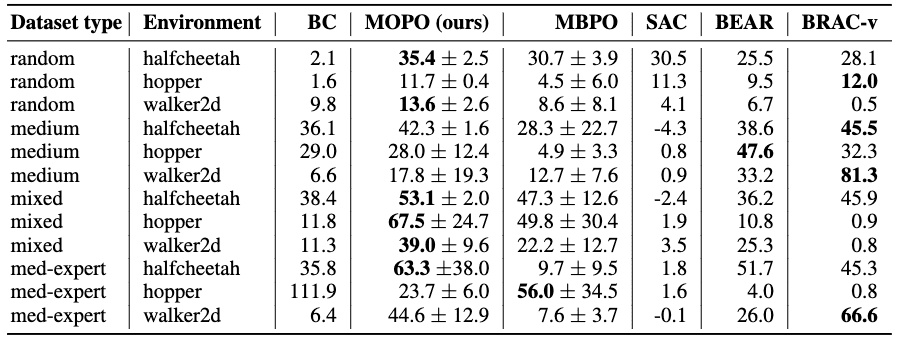
Consequently, in D4RL benchmark, MOPO outperformed others by a significant margin on all the mixed datasets and most of the medium-expert datasets, while also achieving strong performance on all the random datasets.
COMBO: Conservative Offline Model-Based Policy Optimization
Prior model-based offline RL approaches necessitate uncertainty quantification for incorporating conservatism, which is challenging and often unreliable in practice. For instance, uncertainty quantification is hard in these tasks where the agent is required to go further away from the data distribution.
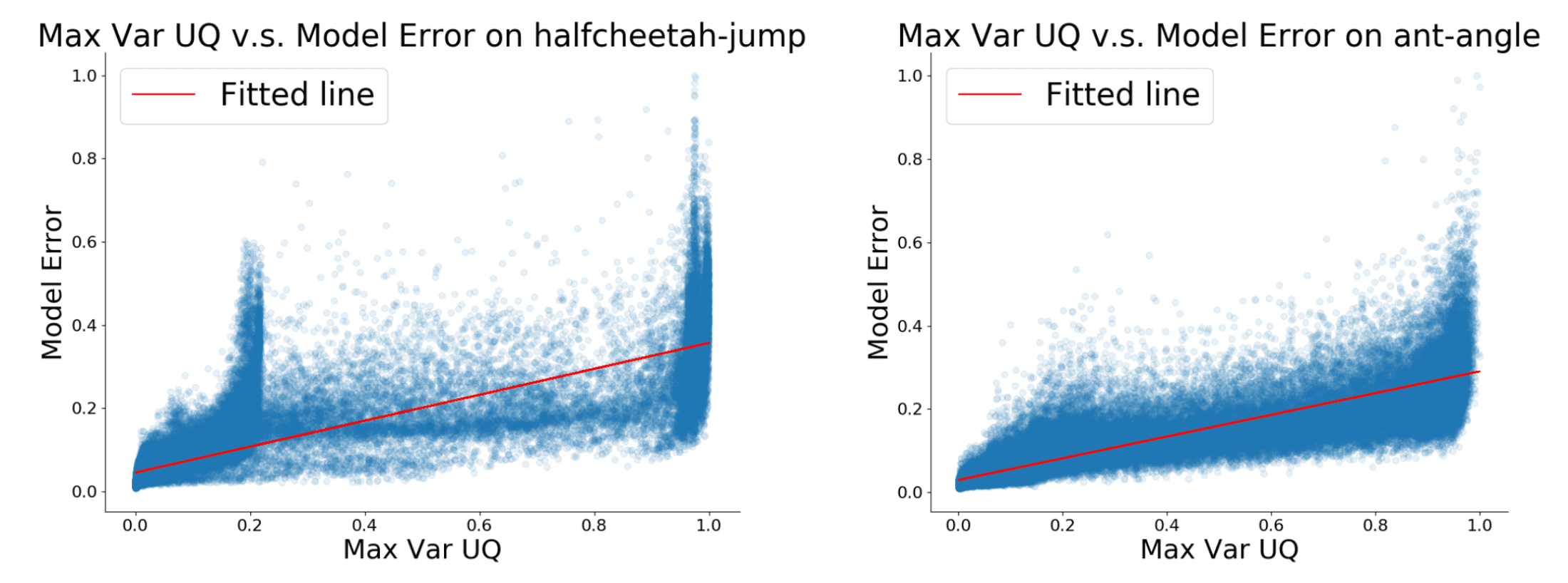
Instead of integrating conservatism into model dynamics, Yu et al., NeurIPS 2021 introduced a model-based version of CQL named conservative offline model-based policy optimization (COMBO), which incorporates conservatism into policy learning without uncertainty estimation.
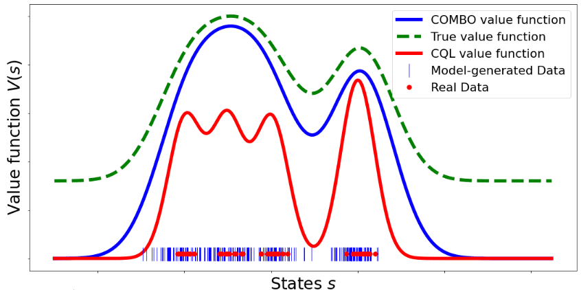
COMBO also learns a single Gaussian dynamics model $\hat{\mathbb{P}} (\mathbf{s}^\prime, r \vert \mathbf{s}, \mathbf{a}) = \mathcal{N}(\mu_\theta (\mathbf{s}, \mathbf{a}), \Sigma_\theta (\mathbf{s}, \mathbf{a}))$ via maximum log-likelihood. With both the offline dataset and simulated data from the model, it learns a conservative (but less than CQL) critic function by penalizing the value function in state-action tuples that are not in the support of the offline dataset.
Conservative Policy Evaluation
Given a policy $\pi$, an offline dataset $\mathcal{D}$, and a learned model $\hat{\mathcal{M}}$ of the MDP, COMBO obtains a conservative estimate of $Q^\pi$ by penealizing the Q-values evaluated on data drawn from a particular state-action distribution that is more likely to be out-of-support while pushing up the Q-values on state-action pairs that are trustworthy, which is implemented by repeating the following recursion:
\[\begin{multline} \hat{Q}^{k + 1} \leftarrow \underset{Q}{\arg \min} \; \alpha \left( \mathbb{E}_{\mathbf{s} \sim d_{\hat{\mathcal{M}}}^\pi, \mathbf{a} \sim \pi (\cdot \vert \mathbf{s})} [Q (\mathbf{s}, \mathbf{a})] - \mathbb{E}_{(\mathbf{s} , \mathbf{a}) \sim \mathcal{D}} [Q (\mathbf{s}, \mathbf{a})] \right) \\ + \frac{1}{2} \mathbb{E}_{(\mathbf{s}, \mathbf{a}, \mathbf{s}^\prime) \sim d_f^\mu} \left[ \left( r (\mathbf{s}, \mathbf{a}) + \gamma \hat{Q}^k (\mathbf{s}^\prime, \mathbf{a}^\prime) - Q(\mathbf{s}, \mathbf{a}) \right)^2 \right] \end{multline}\]where \(d_{\hat{\mathcal{M}}}^\pi(\mathbf{s})\) is the discounted marginal state distribution when executing $\pi$ in the learned model $\hat{\mathcal{M}}$, and $d_f$ is an $f \in [0, 1]$−interpolation between the offline dataset and synthetic rollouts from the model:
\[d_f^\mu (\mathbf{s}, \mathbf{a}) := f \cdot d (\mathbf{s}, \mathbf{a}) + (1 - f) \cdot d_{\hat{\mathcal{M}}}^\mu (\mathbf{s}, \mathbf{a})\]for the rollout distribution $\mu (\mathbf{a} \vert \mathbf{s})$. After learning a conservative critic $\hat{Q}^\pi$, we can improve the policy as:
\[\pi^\prime \leftarrow \underset{\pi}{\arg \max} \; \mathbb{E}_{\mathbf{s} \sim d_{\hat{\mathcal{M}}}^\pi, \mathbf{a} \sim \pi (\cdot \vert \mathbf{s})} \left[ \hat{Q}^\pi (\mathbf{s}, \mathbf{a}) \right]\]

Theoretical Guarantees of COMBO
The following theorem shows that the Q-function $\hat{Q}^\pi$ learned by COMBO lower-bounds the actual Q-function $Q^\pi$ under the initial state distribution $\mu_0$ and any policy $\pi$:
For large $\alpha$, we have: $$ \mathbb{E}_{\mathbf{s} \sim \mu_0, \mathbf{a} \sim \pi (\cdot \vert \mathbf{s})} \left[ \hat{Q}^\pi (\mathbf{s}, \mathbf{a}) \right] \leq \mathbb{E}_{\mathbf{s} \sim \mu_0, \mathbf{a} \sim \pi (\cdot \vert \mathbf{s})} \left[ Q^\pi (\mathbf{s}, \mathbf{a}) \right] $$ where $\mu_0$ is the initial state distribution.
$\mathbf{Proof.}$
Denote the Bellman operator and its sample based counterpart as $\mathcal{B}^\pi$ and $\hat{\mathcal{B}}^\pi$, associated with a single transition $(\mathbf{s}, \mathbf{a}, \mathbf{s}^\prime)$ and $\mathbf{a}^\prime \sim \pi(\cdot \vert \mathbf{s}^\prime)$:
\[\begin{aligned} \mathcal{B}^\pi Q(\mathbf{s}, \mathbf{a}) & := r(\mathbf{s}, \mathbf{a}) + \gamma \mathbb{E}_{\mathbf{s}^\prime \sim \mathbb{P}_\mathcal{S} (\cdot \vert \mathbf{s}, \mathbf{a}), \mathbf{a}^\prime \sim \pi (\cdot \vert \mathbf{s}^\prime)} [Q(\mathbf{s}^\prime, \mathbf{a}^\prime)] \\ \hat{\mathcal{B}}^\pi Q(\mathbf{s}, \mathbf{a}) & := r(\mathbf{s}, \mathbf{a}) + \gamma Q(\mathbf{s}^\prime, \mathbf{a}^\prime) \\ \end{aligned}\]Assuming that the Q-function is tabular, the Q-function found by approximate dynamic programming in iteration $k$, can be obtained by differentiating the update equation with respect to $\hat{Q}^k$:
\[\hat{Q}^{k + 1} (\mathbf{s}, \mathbf{a}) = \left( \hat{\mathcal{B}}^\pi \hat{Q}^k \right) (\mathbf{s}, \mathbf{a}) - \alpha \frac{\rho (\mathbf{s}, \mathbf{a}) - d (\mathbf{s}, \mathbf{a})}{d_f^\mu (\mathbf{s}, \mathbf{a})}\]where $\rho (\mathbf{s}, \mathbf{a}) := d_{\hat{\mathcal{M}}}^\pi (\mathbf{s}) \pi (\mathbf{a} \vert \mathbf{s})$ and $d(\mathbf{s}, \mathbf{a})$ is a dataset distribution. Before proving the main theorem, we first need the following lemma to show that the penalty term of $\hat{Q}^{k + 1}$ is positive in expectation:
For any $f \in [0, 1]$, and any given $\rho (\mathbf{s}, \mathbf{a})$, let $d_f$ be an $f$-interpolation of $\rho$ and $\mathcal{D}$: $$ d_f (\mathbf{s}, \mathbf{a}) := f \cdot d (\mathbf{s}, \mathbf{a}) + (1 - f) \cdot \rho (\mathbf{s}, \mathbf{a}). $$ Define the expected penalty under $\rho (\mathbf{s}, \mathbf{a})$: $$ \nu (\rho, f) := \mathbb{E}_{(\mathbf{s}, \mathbf{a}) \sim \rho (\mathbf{s}, \mathbf{a})} \left[ \frac{\rho (\mathbf{s}, \mathbf{a}) - d (\mathbf{s}, \mathbf{a})}{d_f (\mathbf{s}, \mathbf{a})} \right]. $$ Then, $\nu (\rho, f)$ satisfies:
- $\forall \rho, f: \nu (\rho, f) \geq 0$;
- $\nu (\rho, f)$ is monotone increasing in $f$ for fixed $\rho$;
- $\nu (\rho, f) = 0$ if and only if $\forall \mathbf{s}, \mathbf{a}: \rho (\mathbf{s}, \mathbf{a}) = d(\mathbf{s}, \mathbf{a})$ or $f = 0$;
$\mathbf{Proof.}$
2. Monotone increasing
Note that:
\[\begin{aligned} \nu(\rho, f) &= \sum_{\mathbf{s}, \mathbf{a}} \rho(\mathbf{s}, \mathbf{a}) \left(\frac{\rho(\mathbf{s}, \mathbf{a}) - d(\mathbf{s}, \mathbf{a})}{f \cdot d(\mathbf{s}, \mathbf{a}) + (1 - f) \cdot \rho(\mathbf{s}, \mathbf{a})}\right)\nonumber \\ &= \sum_{\mathbf{s}, \mathbf{a}} \rho(\mathbf{s}, \mathbf{a}) \left(\frac{\rho(\mathbf{s}, \mathbf{a}) - d(\mathbf{s}, \mathbf{a})}{\rho(\mathbf{s}, \mathbf{a}) + f \cdot ( d(\mathbf{s}, \mathbf{a}) - \rho(\mathbf{s}, \mathbf{a}))}\right)\\ \implies \frac{d \nu(\rho, f)}{d f} &= \sum_{\mathbf{s}, \mathbf{a}} \rho(\mathbf{s}, \mathbf{a}) \left(\rho(\mathbf{s}, \mathbf{a}) - d(\mathbf{s}, \mathbf{a})\right)^2 \cdot \left(\frac{1}{(\rho(\mathbf{s}, \mathbf{a})) + f \cdot ( d(\mathbf{s}, \mathbf{a}) - \rho(\mathbf{s}, \mathbf{a}))}\right)^2 \geq 0 \\ &~~~\forall f \in [0, 1]. \end{aligned}\]Since the derivative with respect to $f$ is always positive, this proves the second part (2) of the Lemma.
1. Positivity
Using the monotonic increasing property:
\[\begin{aligned} \forall f \in (0, 1], \; \nu(\rho, f) \geq \nu(\rho, 0) = \sum_{\mathbf{s}, \mathbf{a}} \rho(\mathbf{s}, \mathbf{a}) \frac{\rho(\mathbf{s}, \mathbf{a}) - d(\mathbf{s}, \mathbf{a})}{\rho(\mathbf{s}, \mathbf{a})} &= \sum_{\mathbf{s}, \mathbf{a}} \left( \rho(\mathbf{s}, \mathbf{a}) - d(\mathbf{s}, \mathbf{a}) \right) \\ & = 1 - 1 = 0. \end{aligned}\]3. The necessary and sufficient conditions of $\nu (\rho, f) = 0$
To prove the only if side, assume that $f \neq 0$ and $\rho(\mathbf{s}, \mathbf{a}) \neq d(\mathbf{s}, \mathbf{a})$. When $d(\mathbf{s}, \mathbf{a}) \neq \rho(\mathbf{s}, \mathbf{a})$.
When $d(\mathbf{s}, \mathbf{a}) \neq \rho(\mathbf{s}, \mathbf{a})$, the derivative $\frac{d \nu(\rho,f)}{d f} > 0$ (i.e., strictly positive) and hence the function $\nu(\rho, f)$ is a strictly increasing function of $f$. Therefore, in this case, $\nu(\rho, f) > 0 = \nu(\rho, 0) \; \forall f > 0$. Thus we have shown that if $\rho(\mathbf{s}, \mathbf{a}) \neq d(\mathbf{s}, \mathbf{a})$ and $f > 0$, $\nu(\rho, f) \neq 0$.
\[\tag*{$\blacksquare$}\]Let $\overline{\mathcal{M}}$ be the empirical MDP which uses the empirical transition model based on raw data counts. Then, we will obtain the asymptotic lower-bound by the similar proof of CQL:
Let $\mathcal{P}^\pi$ denote the transition matrix coupled with the policy $\pi$ in the actual MDP and let $\mathcal{S}^\pi := (I − \gamma \mathcal{P}^\pi )^{−1}$. For any $\pi (\mathbf{a} \vert \mathbf{s})$, with probability at least $1 - \delta$: $$ \begin{multline} \forall \mathbf{s}, \mathbf{a}: \; \hat{Q}^\pi(\mathbf{s}, \mathbf{a}) \leq Q^\pi(\mathbf{s}, \mathbf{a}) - \beta \cdot \left[ \mathcal{S}^\pi \left[ \frac{\rho - d}{d_f} \right] \right](\mathbf{s}, \mathbf{a}) + f \left[ \mathcal{S}^\pi \left[ \frac{C_{r, T, \delta} R_{\max}}{(1 - \gamma) \sqrt{\vert \mathcal{D} \vert}} \right] \right](\mathbf{s}, \mathbf{a})\\ + (1 - f) \left[ \mathcal{S}^\pi \left[ \vert r - r_{\hat{\mathcal{M}}} \vert + \frac{ 2 \gamma R_{\max}}{1 - \gamma} \mathrm{TV}(\mathbb{P}, \mathbb{P}_{\hat{\mathcal{M}}}) \right] \right]\!\! (\mathbf{s}, \mathbf{a}). \end{multline} $$
$\mathbf{Proof.}$
Similar to CQL, assume the standard concentration properties of the reward and transition dynamics in the empirical MDP $\overline{\mathcal{M}}$ as follows:
\[\begin{gathered} \left\vert r_{\overline{\mathcal{M}}} (\mathbf{s}, \mathbf{a}) - r (\mathbf{s}, \mathbf{a}) \right\vert \leq \frac{C_{r, \delta}}{\sqrt{\vert \mathcal{D} (\mathbf{s}, \mathbf{a}) \vert}} \\ \left\Vert \mathbb{P}_{\overline{\mathcal{M}}} (\mathbf{s}^\prime \vert \mathbf{s}, \mathbf{a}) - \mathbb{P} (\mathbf{s}^\prime \vert \mathbf{s}, \mathbf{a}) \right\Vert_1 \leq \frac{C_{\mathbb{P}, \delta}}{\sqrt{\vert \mathcal{D} (\mathbf{s}, \mathbf{a}) \vert}} \\ \end{gathered}\]Under this assumption and supposing that $r(\mathbf{s}, \mathbf{a})$ is bounded, as $\vert r(\mathbf{s}, \mathbf{a}) \vert \leq R_{\max}$, we can bound the difference between the empirical Bellman operator \(\mathcal{B}_\overline{\mathcal{M}}^\pi\) and the actual MDP \(\mathcal{B}_\mathcal{M}^\pi\):
\[\begin{aligned} \left\vert \left(\mathcal{B}_{\overline{\mathcal{M}}}^\pi \hat{Q}^k \right) - \left(\mathcal{B}_\mathcal{M}^\pi \hat{Q}^k \right) \right\vert & = \left\vert\left(r_{\overline{\mathcal{M}}}(\mathbf{s}, \mathbf{a}) - r_\mathcal{M}(\mathbf{s}, \mathbf{a})\right)\right. \\ & \left. + \gamma \sum_{\mathbf{s}^\prime \in \mathcal{S}} \left(\mathbb{P}_{\overline{\mathcal{M}}}(\mathbf{s}^\prime \vert \mathbf{s}, \mathbf{a}) - \mathbb{P}_\mathcal{M}(\mathbf{s}^\prime \vert \mathbf{s},\mathbf{a})\right) \mathbb{E}_{\pi(\mathbf{a}^\prime \vert \mathbf{s}^\prime)}\left[\hat{Q}^k(\mathbf{s}^\prime, \mathbf{a}^\prime)\right]\right\vert \\ & \leq \left\vert r_{\overline{\mathcal{M}}}(\mathbf{s}, \mathbf{a}) - r_\mathcal{M}(\mathbf{s}, \mathbf{a})\right\vert \\ & + \gamma \left\vert \sum_{\mathbf{s}^\prime} \left(\mathbb{P}_{\overline{\mathcal{M}}}(\mathbf{s}^\prime \vert \mathbf{s}, \mathbf{a}) - \mathbb{P}_\mathcal{M}(\mathbf{s}^\prime \vert \mathbf{s},\mathbf{a})\right) \mathbb{E}_{\pi(\mathbf{a}^\prime \vert \mathbf{s}^\prime)}\left[\hat{Q}^k(\mathbf{s}^\prime , \mathbf{a}^\prime)\right]\right\vert \\ & \leq \frac{C_{r, \delta} + \gamma C_{\mathbb{P}, \delta} 2R_{\max} / (1 - \gamma)}{\sqrt{\vert \mathcal{D}(\mathbf{s}, \mathbf{a}) \vert}}. \end{aligned}\]Therefore, we have:
\[\forall (\mathbf{s}, \mathbf{a}) \in \mathcal{S} \times \mathcal{A}: \;\left\vert \left(\mathcal{B}_{\overline{\mathcal{M}}}^\pi \hat{Q}^k \right) - \left(\mathcal{B}_\mathcal{M}^\pi \hat{Q}^k \right) \right\vert \leq \frac{C_{r, \mathbb{P}, \delta} R_{\max}}{(1 - \gamma) \sqrt{\vert \mathcal{D}(\mathbf{s}, \mathbf{a}) \vert}}\]for some constant $C_{r, \mathbb{P}, \delta} > 0$. Subsequently, to obtain a bound on the error between the bellman backup induced by the learned dynamics model and the learned reward \(\mathcal{B}_\hat{\mathcal{M}}^\pi\) and the actual Bellman backup \(\mathcal{B}_\mathcal{M}^\pi\), note that:
\[\begin{aligned} \left\vert \left(\mathcal{B}_{\hat{\mathcal{M}}}^\pi \hat{Q}^k \right) - \left(\mathcal{B}_{\mathcal{M}}^\pi \hat{Q}^k \right) \right\vert &= \left\vert \left(r_\hat{\mathcal{M}} (\mathbf{s}, \mathbf{a}) - r_\mathcal{M} (\mathbf{s}, \mathbf{a}) \right) \right. \\ & \left. + \gamma \sum_{\mathbf{s}^\prime \in \mathcal{S}} \left(\mathbb{P}_{\hat{\mathcal{M}}}(\mathbf{s}^\prime \vert \mathbf{s}, \mathbf{a}) - \mathbb{P}_\mathcal{M} (\mathbf{s}^\prime \vert \mathbf{s}, \mathbf{a})\right) \mathbb{E}_{\pi(\mathbf{a}^\prime \vert \mathbf{s}^\prime)}\left[\hat{Q}^k(\mathbf{s}^\prime, \mathbf{a}^\prime)\right]\right\vert \\ &\leq \vert r_{\hat{\mathcal{M}}}(\mathbf{s}, \mathbf{a}) - r_\mathcal{M}(\mathbf{s}, \mathbf{a}) \vert + \gamma \frac{2 R_{\max}}{1 - \gamma} \mathrm{TV}(\mathbb{P}, \mathbb{P}_{\hat{\mathcal{M}}}) \end{aligned}\]Using these error bounds, now we can prove that the asymptotic Q-function learned by COMBO lower-bounds the actual Q-function of any $\pi$ with high probability for a large enough $\alpha \geq 0$.
\[\begin{aligned} \hat{Q}^{k+1}(\mathbf{s}, \mathbf{a}) &= \left(\hat{\mathcal{B}}^\pi \hat{Q}^k\right)(\mathbf{s}, \mathbf{a}) - \alpha \frac{\rho(\mathbf{s}, \mathbf{a}) - d(\mathbf{s}, \mathbf{a})}{d_f(\mathbf{s}, \mathbf{a})}\\ &= f \left(\mathcal{B}^\pi_{\overline{\mathcal{M}}} \hat{Q}^k \right) (\mathbf{s}, \mathbf{a}) + (1 - f) \left(\mathcal{B}^\pi_{\hat{\mathcal{M}}} \hat{Q}^k \right) (\mathbf{s}, \mathbf{a}) - \alpha \frac{\rho(\mathbf{s}, \mathbf{a}) - d(\mathbf{s}, \mathbf{a})}{d_f(\mathbf{s}, \mathbf{a})}\\ &= \left(\mathcal{B}^\pi \hat{Q}^k\right)(\mathbf{s}, \mathbf{a}) - \alpha \frac{\rho(\mathbf{s}, \mathbf{a}) - d(\mathbf{s}, \mathbf{a})}{d_f(\mathbf{s}, \mathbf{a})} + (1 - f) \left({\mathcal{B}_{\hat{\mathcal{M}}}}^\pi \hat{Q}^k - {\mathcal{B}}^\pi \hat{Q}^k \right)(\mathbf{s}, \mathbf{a})\\ &+ f \left({\mathcal{B}_{\overline{\mathcal{M}}}}^\pi \hat{Q}^k - {\mathcal{B}}^\pi \hat{Q}^k \right)(\mathbf{s}, \mathbf{a}) \end{aligned}\]Therefore:
\[\forall \mathbf{s}, \mathbf{a}: \; \hat{Q}^{k+1} \leq \left(\mathcal{B}^\pi \hat{Q}^k\right) - \alpha \frac{\rho - d}{d_f} + (1 - f) \left[\vert r_{\hat{\mathcal{M}}} - r_\mathcal{M} \vert + \frac{2 \gamma R_{\max}}{1 - \gamma} \mathrm{TV}(\mathbb{P}, \mathbb{P}_{\hat{\mathcal{M}}}) \right] + f \frac{C_{r, \mathbb{P}, \delta} R_{\max}}{(1 - \gamma) \sqrt{\vert \mathcal{D} \vert}}\]By substituting $\hat{Q}$ by the fixed point $\hat{Q}^\pi$ and the definition of Bellman operator, we obtain:
\[\begin{multline} \hat{Q}^\pi(\mathbf{s}, \mathbf{a}) \leq \underbrace{ \mathcal{S}^\pi r_{\mathcal{M}}}_{= Q^\pi(\mathbf{s}, \mathbf{a})} - \alpha \left[ \mathcal{S}^\pi \left[ \frac{\rho - d}{d_f} \right] \right](\mathbf{s}, \mathbf{a}) + f \left[ \mathcal{S}^\pi \left[ \frac{C_{r, \mathbb{P}, \delta} R_{\max}}{(1 - \gamma) \sqrt{\vert \mathcal{D} \vert}} \right] \right](\mathbf{s}, \mathbf{a})\\ + (1 - f) \left[ \mathcal{S}^\pi \left[ \vert r - r_{\hat{\mathcal{M}}} \vert + \frac{ 2 \gamma R_{\max}}{1 - \gamma} \mathrm{TV}(\mathbb{P}, \mathbb{P}_{\hat{\mathcal{M}}}) \right] \right] (\mathbf{s}, \mathbf{a}) \end{multline}\] \[\tag*{$\blacksquare$}\]Finally, we use the result and proof technique from this proposition to prove the main theorem. Note that:
\[\begin{aligned} \hat{Q}^{k+1}(\mathbf{s}, \mathbf{a}) & = \left(\hat{\mathcal{B}}^\pi \hat{Q}^k\right)(\mathbf{s}, \mathbf{a}) - \alpha \frac{\rho(\mathbf{s}, \mathbf{a}) - d(\mathbf{s}, \mathbf{a})}{d_f(\mathbf{s}, \mathbf{a})} \\ & = \left(\mathcal{B}^\pi_{\hat{\mathcal{M}}} \hat{Q}^k \right)(\mathbf{s}, \mathbf{a}) - \alpha \frac{\rho(\mathbf{s}, \mathbf{a}) - d(\mathbf{s}, \mathbf{a})}{d_f(\mathbf{s}, \mathbf{a})} + f \underbrace{\left(\mathcal{B}^\pi_{\overline{\mathcal{M}}} - \mathcal{B}^\pi_{\hat{\mathcal{M}}} \hat{Q}^k \right)(\mathbf{s}, \mathbf{a})}_{:= \Delta(\mathbf{s}, \mathbf{a})} \end{aligned}\]By controlling $\Delta (\mathbf{s}, \mathbf{a})$ using the pointwise triangle inequality:
\[\forall \mathbf{s}, \mathbf{a}, \; \left\vert \mathcal{B}^\pi_{\overline{\mathcal{M}}} \hat{Q}^k - \mathcal{B}^\pi_{\hat{\mathcal{M}}} \hat{Q}^k \right\vert \leq \left\vert \mathcal{B}^\pi \hat{Q}^k - \mathcal{B}^\pi_{\hat{\mathcal{M}}} \hat{Q}^k \right\vert + \left\vert \mathcal{B}^\pi_{\overline{\mathcal{M}}} \hat{Q}^k - \mathcal{B}^\pi \hat{Q}^k \right\vert\]and then interating the backup \(\mathcal{B}_{\hat{\mathcal{M}}}^\pi\) to its fixed point and finally noting that
\[\rho (\mathbf{s}, \mathbf{a}) = \left( (\mu \cdot \pi)^\top \mathcal{S}_{\hat{\mathcal{M}}}^\pi \right) (\mathbf{s}, \mathbf{a})\]we obtain:
\[\mathbb{E}_{\mu, \pi}[\hat{Q}^\pi(\mathbf{s}, \mathbf{a})] \leq \mathbb{E}_{\mu, \pi}[Q^\pi_{\hat{\mathcal{M}}}(\mathbf{s}, \mathbf{a})] - \alpha~ \mathbb{E}_{\rho(\mathbf{s}, \mathbf{a})}\left[\frac{\rho(\mathbf{s}, \mathbf{a}) - d(\mathbf{s}, \mathbf{a})}{d_f(\mathbf{s}, \mathbf{a})}\right] + C\]where $C$ is a term independent of $\alpha$ that correspond to the additional positive error terms obtained by iterating \(\vert \mathcal{B}_\mathcal{M}^\pi \hat{Q}^k - \mathcal{B}_{\hat{\mathcal{M}}}^\pi \vert\) and \(\vert \mathcal{B}_\overline{\mathcal{M}}^\pi \hat{Q}^k - \mathcal{B}_{\mathcal{M}}^\pi \vert\), which can be bounded similar to the proof of the previous proposition.
By replacing the model Q-function \(\mathbb{E}_{\mu, \pi}[Q^\pi_{\hat{\mathcal{M}}}(\mathbf{s}, \mathbf{a})]\) with the actual Q-function \(\mathbb{E}_{\mu, \pi}[Q^\pi(\mathbf{s}, \mathbf{a})]\), and adding an error term corresponding to model error, we finally obtain:
\[\mathbb{E}_{\mu, \pi} \left[ \hat{Q}^\pi (\mathbf{s}, \mathbf{a}) \right] \leq \mathbb{E}_{\mu, \pi} \left[ Q^\pi (\mathbf{s}, \mathbf{a}) \right] + C - \alpha \underbrace{\mathbb{E}_{\rho (\mathbf{s}, \mathbf{a})} \left[ \frac{\rho (\mathbf{s}, \mathbf{a}) - d (\mathbf{s}, \mathbf{a})}{d_f (\mathbf{s}, \mathbf{a})} \right]}_{= \nu (\rho, f) > 0}\]Hence, by choosing $\alpha$ large enough, we obtain the desired lower bound guarantee.
\[\tag*{$\blacksquare$}\]This theorem suggests that COMBO is less conservative in that it does not underestimate the value function at every state in the dataset like CQL:
\[\forall \mathbf{s} \in \mathcal{D}: \; \hat{V}_{\texttt{CQL}}^\pi (\mathbf{s}) \leq V^\pi (\mathbf{s})\]whereas the COMBO bound is only valid in expectation of the value function over the initial state distribution and the value function at a given state may not be a lower-bound:
\[\mathbb{E}_{\mathbf{s} \sim \mu_0 (\mathbf{s})} \left[ \hat{V}_{\texttt{COMBO}}^\pi (\mathbf{s}) \right] \leq \mathbb{E}_{\mathbf{s} \sim \mu_0 (\mathbf{s})} \left[ V^\pi (\mathbf{s}) \right]\]And theoretically, they demonstrated that COMBO will be less conservative than CQL when the action probabilities under learned policy $\pi(\mathbf{a}\vert \mathbf{s})$ and the probabilities under the behavior policy $\pi_\beta (\mathbf{a} \vert \mathbf{s})$ are closer together on state-action tuples sampled from the model and actions from $\pi$, $d_{\hat{\mathcal{M}}} (\mathbf{s}) \pi(\mathbf{a} \vert \mathbf{s})$, than they are on states from the dataset and actions from $\pi$, $d_{\overline{\mathcal{M}}} (\mathbf{s}) \pi(\mathbf{a} \vert \mathbf{s})$:
Let $\overline{\mathcal{M}}$ be the empirical MDP which uses the empirical transition model based on raw data counts. And assume that: $$ \mathbb{E}_{\mathbf{s} \sim d_{\hat{\mathcal{M}}} (\mathbf{s}), \mathbf{a} \sim \pi (\mathbf{a} \vert \mathbf{s})} \left[ \frac{\pi (\mathbf{a} \vert \mathbf{s})}{\pi_\beta (\mathbf{a} \vert \mathbf{s})} \right] \leq \mathbb{E}_{\mathbf{s} \sim d_{\overline{\mathcal{M}}} (\mathbf{s}), \mathbf{a} \sim \pi (\mathbf{a} \vert \mathbf{s})} \left[ \frac{\pi (\mathbf{a} \vert \mathbf{s})}{\pi_\beta (\mathbf{a} \vert \mathbf{s})} \right] $$ Then, we have: $$ \mathbb{E}_{\mathbf{s} \sim d_{\overline{\mathcal{M}}} (\mathbf{s}), \mathbf{a} \sim \pi (\mathbf{a} \vert \mathbf{s})} \left[ \hat{Q}_{\texttt{COMBO}}^\pi (\mathbf{s}, \mathbf{a}) \right] \geq \mathbb{E}_{\mathbf{s} \sim d_{\overline{\mathcal{M}}} (\mathbf{s}), \mathbf{a} \sim \pi (\mathbf{a} \vert \mathbf{s})} \left[ \hat{Q}_{\texttt{CQL}}^\pi (\mathbf{s}, \mathbf{a}) \right] $$
$\mathbf{Proof.}$
From the proof in CQL paper, note that:
\[\hat{Q}_{\texttt{CQL}}^\pi (\mathbf{s}, \mathbf{a}) := Q^\pi (\mathbf{s}, \mathbf{a}) - \alpha \frac{\pi(\mathbf{a} \vert \mathbf{s}) - \pi_\beta (\mathbf{a} \vert \mathbf{s})}{\pi_\beta (\mathbf{a} \vert \mathbf{s})}\]Denote $\rho (\mathbf{s}, \mathbf{a}) := d_{\hat{\mathcal{M}}} (\mathbf{s}) \pi (\mathbf{a} \vert \mathbf{s})$. In this proof, we only consider $f = 1$ case, as $f \neq 1$ gives the desired result too, but it will be hard to interpret terms appear in the final inequality.
Thus for $f = 1$ (that is, $d_f = d^{\pi_\beta}$), re-write the inequality:
\[\begin{aligned} & \mathbb{E}_{\mathbf{s} \sim d_{\overline{\mathcal{M}}} (\mathbf{s}), \mathbf{a} \sim \pi (\mathbf{a} \vert \mathbf{s})} \left[ \hat{Q}_{\texttt{COMBO}}^\pi (\mathbf{s}, \mathbf{a}) \right] \geq \mathbb{E}_{\mathbf{s} \sim d_{\overline{\mathcal{M}}} (\mathbf{s}), \mathbf{a} \sim \pi (\mathbf{a} \vert \mathbf{s})} \left[ \hat{Q}_{\texttt{CQL}}^\pi (\mathbf{s}, \mathbf{a}) \right] \\ \implies & \sum_{\mathbf{s}, \mathbf{a}} d_{\overline{\mathcal{M}}} (\mathbf{s}) \pi (\mathbf{a} \vert \mathbf{s}) \hat{Q}_{\texttt{COMBO}}^\pi (\mathbf{s}, \mathbf{a}) \geq \sum_{\mathbf{s}, \mathbf{a}} d_{\overline{\mathcal{M}}} (\mathbf{s}) \pi (\mathbf{a} \vert \mathbf{s}) \hat{Q}_{\texttt{CQL}}^\pi (\mathbf{s}, \mathbf{a}) \\ \implies & \alpha \sum_{\mathbf{s}, \mathbf{a}} d_{\overline{\mathcal{M}}} (\mathbf{s}) \pi (\mathbf{a} \vert \mathbf{s}) \left( \frac{\rho (\mathbf{s}, \mathbf{a} - d^{\pi_\beta} (\mathbf{s}) \pi_\beta (\mathbf{a} \vert \mathbf{s}))}{ d^{\pi_\beta} (\mathbf{s}) \pi_\beta (\mathbf{a} \vert \mathbf{s}) } \right) \geq \alpha \sum_{\mathbf{s}, \mathbf{a}} d_{\overline{\mathcal{M}}} (\mathbf{s}) \pi (\mathbf{a} \vert \mathbf{s}) \left( \frac{\pi(\mathbf{a} \vert \mathbf{s}) - \pi_\beta (\mathbf{a} \vert \mathbf{s})}{\pi_\beta (\mathbf{a} \vert \mathbf{s})} \right). \end{aligned}\]In the LHS, by adding and subtracting $d^{\pi_\beta} (\mathbf{s}) \pi (\mathbf{a} \vert \mathbf{s})$ from the numerator:
\[\begin{aligned} & \sum_{\mathbf{s}, \mathbf{a}} d_{\overline{\mathcal{M}}}(\mathbf{s}, \mathbf{a}) \left( \frac{\rho(\mathbf{s}, \mathbf{a}) - d^{\pi_\beta}(\mathbf{s}) \pi_\beta(\mathbf{a} \vert \mathbf{s})}{d^{\pi_\beta}(\mathbf{s}) \pi_\beta(\mathbf{a} \vert \mathbf{s})} \right)\\ &= \sum_{\mathbf{s}, \mathbf{a}} d_{\overline{\mathcal{M}}}(\mathbf{s}, \mathbf{a}) \left( \frac{\rho(\mathbf{s}, \mathbf{a}) - d^{\pi_\beta}(\mathbf{s}) \pi(\mathbf{a}\vert\mathbf{s}) + d^{\pi_\beta}(\mathbf{s}) \pi(\mathbf{a}\vert\mathbf{s}) - d^{\pi_\beta}(\mathbf{s}) \pi_\beta(\mathbf{a} \vert \mathbf{s})}{d^{\pi_\beta}(\mathbf{s}) \pi_\beta(\mathbf{a}|\mathbf{s})} \right) \\ &= \underbrace{\sum_{\mathbf{s}, \mathbf{a}} d_{\overline{\mathcal{M}}}(\mathbf{s}, \mathbf{a}) \frac{\pi(\mathbf{a} \vert \mathbf{s}) - \pi_\beta(\mathbf{a} \vert \mathbf{s})}{\pi_\beta(\mathbf{a} \vert \mathbf{s})}}_{(1)} + \sum_{\mathbf{s}, \mathbf{a}} d_{\overline{\mathcal{M}}}(\mathbf{s}, \mathbf{a}) \cdot \frac{d_{\hat{\mathcal{M}}} (\mathbf{s}) - d^{\pi_\beta}(\mathbf{s})}{d^{\pi_\beta}(\mathbf{s})} \cdot \frac{\pi(\mathbf{a}|\mathbf{s})}{\pi_\beta(\mathbf{a} \vert \mathbf{s})} \end{aligned}\]Therefore, the inequality of the theorem is satisfied when the second term above is negative. First, note that $d^{\pi_\beta} (\mathbf{s}) = d_{\overline{\mathcal{M}}} (\mathbf{s})$ which results in a cancellation. Then, by re-aranging the second term into expectations gives us the desired result.
\[\tag*{$\blacksquare$}\]Note that COMBO’s objective only penalizes Q-values under $(\mathbf{s}, \mathbf{a}) \sim d_{\hat{\mathcal{M}}} (\mathbf{s}) \pi (\mathbf{a} \vert \mathbf{s})$, which are expected to primarily consist of out-of-distribution states generated from model rollouts, and does not penalize the Q-value at states drawn from the dataset. Consequently, the condition inequality is likely to be negative, making COMBO less conservative than CQL in practice.
Empirical Results
In the D4RL benchmark, COMBO achieves the best performance in 9 out of 12 settings and comparable results in 1 of the remaining 3. While it is generally known that model-based offline methods are typically performant on datasets with diverse state-action distributions (random, medium-replay) and model-free approaches perform better on datasets with narrow distributions (medium, medium-expert), COMBO performs well across all dataset types. This suggests that COMBO is robust to different dataset types.

And COMBO significantly outperforms MOPO, MOReL and CQL in tasks requiring the agent to solve different tasks than those solved by the behavior policy. This demonstrates that COMBO achieves better generalization by being less conservative than CQL, and more robust than MOReL and MOPO.

References
[1] Kidambi et al., “MOReL: Model-Based Offline Reinforcement Learning”, NeurIPS 2020
[2] Yu et al., “MOPO: Model-based Offline Policy Optimization”, NeurIPS 2020
[3] Yu et al., “COMBO: Conservative Offline Model-Based Policy Optimization”, NeurIPS 2021

Leave a comment