[RL] Inverse Reinforcement Learning (IRL)
For imitation learning, I previously discussed behavior cloning, which directly imitates the expert’s policy through supervised learning. Inverse reinforcement learning, also referred to as inverse optimal control, is another methodology that indirectly achieves imitation. Unlike traditional reinforcement learning, which requires explicit reward functions to guide an agent’s actions, IRL accomplishes imitation by learning the expert’s reward function from observed behaviors.
Motivation
Inverse reinforcement learning is deeply connected to the core issues of theoretical biology, econometrics, and other scientific fields that examine reward-driven behavior.
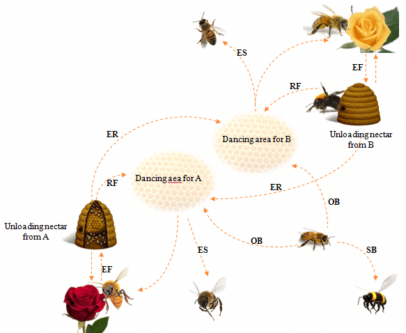
Example: bee foraging
For instance, consider constructing models of bee foraging where each flower is a saturating function of nectar content. A bee might evaluate nectar ingestion in relation to flight distance, time, and risks from wind and predators, but determining the relative weight of these factors a priori is not straightforward. In such cases, inverse reinforcement learning enables us to identify the relative weights of these factors.
Example: self-driving car
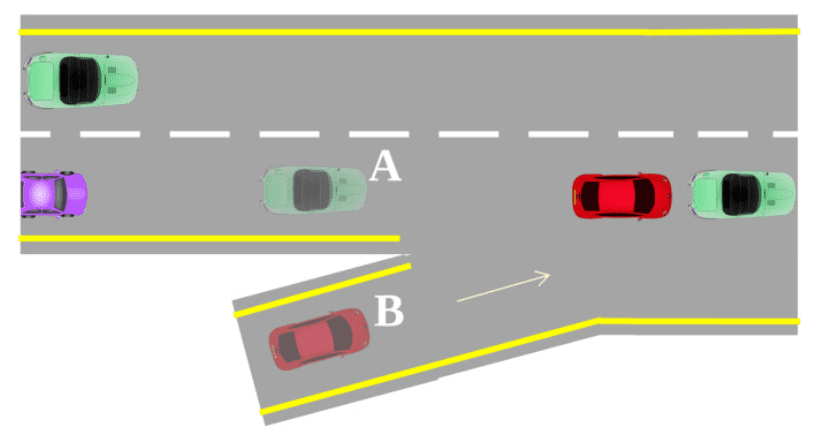
In the context of human behavior, consider a self-driving car in role $\textrm{B}$ as depicted in the following figure. To merge safely into a congested freeway, it may model the behavior of the car in role $\textrm{A}$, which represents the immediate traffic. By analyzing previously collected trajectories of cars in roles $\textrm{A}$ and $\textrm{B}$ on freeway entry ramps, we can infer the safety and speed preferences of a typical driver approaching this complex merge.
Formulation
Consequently, IRL simply inverts the RL problem:
Let \(\mathcal{D} = \{ \tau_i = (\mathbf{s}_0^i, \mathbf{a}_0^i, \cdots, \mathbf{s}_{T_i}^i, \mathbf{a}_{T_i}^i) \}_{i=1}^N\) be the demonstrations of the expert \(\pi^*\) under the MDP environment $\mathcal{M} \setminus \mathbf{R}$ where the reward function $\mathbf{R}$ is unknown. Inverse RL attempts to determine $\mathbf{R}$ that best explains either an expert \(\pi^*\) if given or the observed behavior in the form of demonstrated trajectories $\mathcal{D}$.
To find the optimal reward $\mathbf{R}$, the general IRL methods parametrize the reward function $\mathbf{R}$; most algorithms express $\mathbf{R}$ as a linear combination of features $\boldsymbol{\phi}$:
\[\mathbf{R}(\mathbf{s}, \mathbf{a}) = \theta_1 \phi_1 (\mathbf{s}, \mathbf{a}) + \cdots + \theta_D \phi_D (\mathbf{s}, \mathbf{a}) = \boldsymbol{\theta} \cdot \boldsymbol{\phi}\]where feature functions $\boldsymbol{\phi}$ is given in priori to model a facet of the expert’s preferences. Then the IRL problem reduces to finding the values of the weights $\boldsymbol{\theta}$.
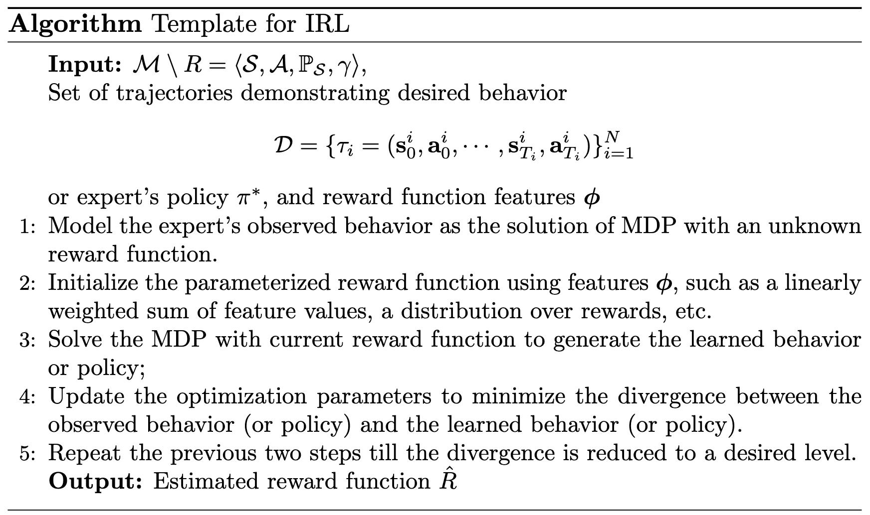
And many fundamental IRL methods fit the following template of key steps (though not universally):
Challenge: Reward Ambiguity
A common and important challenge of IRL is that the IRL problem is its ill-posed nature, as multiple reward functions (including highly degenerate ones, such as those assigning zero rewards universally) can account for the expert’s behavior. This arises because the input of algorithm typically consists of a finite and limited set of trajectories (or a policy), and many reward functions within the entire space of possible functions can produce policies that replicate the observed demonstrations. Consequently, inverse reinforcement learning is suffers from this reward ambiguity.
Max Margin IRL
The max-margin method was the first class of IRL algorithms and attempts to estimate rewards that maximize the margin between the optimal policy (or value function) and all other policies (or value functions).
Original IRL Algorithm
The first IRL algorithm within MDP formulation was introduced by Ng et al. 2000. They essentially formulated the IRL problem as a linear programming procedure, with some constraints corresponding to the optimal condition. The original pape primarily addresses 3 cases in the IRL problem formulation:
(1) Finite-state MDP with known optimal policy.
(2) Infinite-state MDP with known optimal policy.
(3) Infinite-state MDP with unknown optimal policy, but sample trajectory are given.
Finite state space with known optimal policy
In the simplest scenario, assume that a state space $\mathcal{S}$ of the MDP is finite and the optimal policy $\pi$ is known. Then, given $\pi (\mathbf{s}) = \mathbf{a}_1$, the policy $\pi$ is optimal if and only if the reward function $\mathbf{R}$ satisfies:
\[\begin{aligned} & Q^\pi (\mathbf{s}, \mathbf{a}_1) \geq Q^\pi (\mathbf{s}, \mathbf{a}) \quad \forall \mathbf{a} \in \mathcal{A} \setminus \mathbf{a}_1 \\ \Leftrightarrow & \; \mathbf{P}^{\mathbf{a}_1} \mathbf{V}^\pi \geq \mathbf{P}^{\mathbf{a}} \mathbf{V}^\pi \\ \Leftrightarrow & \; \mathbf{P}^{\mathbf{a}_1} (\mathbf{I} - \gamma \mathbf{P}^{\mathbf{a}_1})^{-1} \mathbf{R} \geq \mathbf{P}^{\mathbf{a}} (\mathbf{I} - \gamma \mathbf{P}^{\mathbf{a}_1})^{-1} \mathbf{R} \\ \Leftrightarrow & \; (\mathbf{P}^{\mathbf{a}_1} - \mathbf{P}^{\mathbf{a}} )(\mathbf{I} - \gamma \mathbf{P}^{\mathbf{a}_1})^{-1} \mathbf{R} \geq 0 \\ \end{aligned}\]where $\mathbf{P}^{\mathbf{a}_1}$ is the transition probability matrix for taking the optimal action $\mathbf{a}_1$, and $\mathbf{a}$ represents actions produced by any sub-optimal policies. Note that the solution set includes $\mathbf{R} = 0$ along with numerous other solutions. To address this ambiguity, the authors proposed a linear programming with a penalty term:
\[\begin{array}{cl} \max & \left\{\sum_{i=1}^N \min _{\mathbf{a} \in \mathcal{A} \setminus \mathbf{a}_1}\left\{\left(\mathbf{P}_i^{\mathbf{a}_1} -\mathbf{P}_i^\mathbf{a}\right)\left(\mathbf{I}-\gamma \mathbf{P}^{\mathbf{a}_1}\right)^{-1} \mathbf{R}\right\}-\lambda \Vert \mathbf{R} \Vert_1 \right\} \\ \text { s.t. } & \left(\mathbf{P}^{\mathbf{a}_1}-\mathbf{P}^\mathbf{a}\right)\left(\mathbf{I} -\gamma \mathbf{P}^{\mathbf{a}_1}\right)^{-1} \mathbf{R} \geq 0 \quad \text { and } \quad\left\vert \mathbf{R}_i\right\vert \leq R_{\max } \end{array}\]where the inner-side of $\max$ term is the return difference between the best and second best policy, and the penalty term prevents solutions from that mainly assign small rewards to most states and large rewards to a few states.
Infinite state space with known optimal policy
For problems with an infinite state space $\mathcal{S}$, searching through all reward functions is impractical. Instead, the reward function $R$ is approximated by a linear combination of all useful features $\boldsymbol{\phi}$:
\[R (\mathbf{s}) = \alpha_1 \phi_1 (\mathbf{s}) + \alpha_2 \phi_2 (\mathbf{s}) + \cdots + \alpha_D \phi_D (\mathbf{s}) = \boldsymbol{\alpha} \cdot \boldsymbol{\phi} (\mathbf{s})\]where $D$ is the number of useful features in the reward function and $\alpha$ are the parameters to be learned during the algorithm. Then, the value function $V^\pi (\mathbf{s})$ can be represented as a linear combination of feature expectations:
\[V^\pi (\mathbf{s}) = \alpha_1 \mu_1 (\pi, \mathbf{s}) + \alpha_2 \mu_2 (\pi, \mathbf{s}) + \cdots + \alpha_D \mu_D (\pi, \mathbf{s}) = \boldsymbol{\alpha} \cdot \boldsymbol{\mu} (\pi, \mathbf{s})\]where $\mu$ is the feature expectation defined by:
\[\mu_i (\pi, \mathbf{s}) = \mathbb{E}_\pi \left[ \sum_{t=0}^\infty \gamma^t \phi_i (\mathbf{s}_t) \middle\vert \mathbf{s}_0 = \mathbf{s} \right]\]Again, for a policy $\pi$ to be optimal under the infinite state assumption, the following constraint must hold:
\[\mathbb{E}_{\mathbf{s}^\prime \sim \mathbb{P}_\mathcal{S} (\cdot \vert \mathbf{s}, \mathbf{a}_1)} \left[ V^\pi (\mathbf{s}^\prime) \right] \geq \mathbb{E}_{\mathbf{s}^\prime \sim \mathbb{P}_\mathcal{S} (\cdot \vert \mathbf{s}, \mathbf{a})} \left[ V^\pi (\mathbf{s}^\prime) \right] \quad \forall \mathbf{s} \in \mathcal{S} \textrm{ and } \mathbf{a} \in \mathcal{A} \setminus \mathbf{a}_1\]where $\mathbf{a}_1 = \pi (\mathbf{s})$. Again, since the solution set includes degenerate solution $\mathbf{R} = \mathbf{0}$. Therefore, the optimization problem is relaxed with a penalty when the constraint is violated:
\[\begin{array}{cl} \max & \left\{\sum_{\mathbf{s} \in \mathcal{S}_0} \min _{\mathbf{a} \in \mathcal{A} \setminus \mathbf{a}_1}\left\{ p \left( \mathbb{E}_{\mathbf{s}^\prime \sim \mathbb{P}_\mathcal{S} (\cdot \vert \mathbf{s}, \mathbf{a}_1)} \left[ V^\pi (\mathbf{s}^\prime) \right] - \mathbb{E}_{\mathbf{s}^\prime \sim \mathbb{P}_\mathcal{S} (\cdot \vert \mathbf{s}, \mathbf{a})} \left[ V^\pi (\mathbf{s}^\prime) \right] \right) \right\} \right\} \\ \text { s.t. } & \vert \alpha_i \vert \leq 1, i = 1, \cdots, D \end{array}\]where $p (x)$ is a penalty function and $c$ is a positive constant:
\[p(x) = \begin{cases} x & \quad \textrm{ if } x \geq 0 \\ cx & \quad \textrm{ otherwise } \end{cases}\]Note that evaluating the infinite state space is challenging; therefore, a subsample of $\mathcal{S} \setminus \mathcal{S}_0$ is used.
From sampled trajectories
Now, in a more realistic case, we have access to the optimal policy $\pi$ only through a set of actual trajectories. Let $\mathcal{D}$ be a fixed initial state distribution. The objective of the IRL algorithms is therefore to find $R$ such that the unknown policy $\pi$ maximizes $\mathbb{E}_{\mathbf{s}_0 \sim \mathcal{D}} \left[ V^\pi (\mathbf{s}_0) \right]$. From the $m$ sampled trajectory of states \(\{ \mathbf{s}_t^j \vert t = 1, \cdots \}_{j=1}^m\), we can estimate the feature expectation by Monte Carlo estimation:
\[\mu_i (\pi, \mathbf{s}) \approx \hat{\mu}_i (\mathbf{s}) = \frac{1}{m} \sum_{j=1}^m \sum_{t=0} \gamma^t \phi_i (\mathbf{s}_t) \textrm{ where } \mathbf{s}_0 = \mathbf{s}\]and thus the value function $V^\pi$ can be approximated as:
\[V^\pi (\mathbf{s}) \approx \hat{V}^\pi (\mathbf{s}) = \alpha_1 \hat{\mu}_1 (\mathbf{s}) + \alpha_2 \hat{\mu}_2 (\mathbf{s}) + \cdots + \alpha_D \hat{\mu}_D (\mathbf{s}) = \boldsymbol{\alpha} \cdot \hat{\boldsymbol{\mu}} (\mathbf{s})\]Then, given a policy set \(\{ \pi_1, \cdots, \pi_k \}\), the following optimization can be performed:
\[\begin{array}{cl} \max & \sum_{i=1}^k p \left( \hat{V}^{\pi} (\mathbf{s}_0) - \hat{V}^{\pi_i} (\mathbf{s}_0) \right)\\ \text { s.t. } & \vert \alpha_i \vert \leq 1, i = 1, \cdots, D \end{array}\]This optimization yields a new configuration of the $\alpha_i$s, and consequently a new reward function $R = \boldsymbol{\alpha} \cdot \boldsymbol{\phi}$. We then determine a policy $\pi_{k + 1}$ that maximizes \(V^\pi (\mathbf{s}_0)\) under $R$, and add $\pi_{k + 1}$ to the current policy set. The algorithm is then repeated for a set number of iterations or until a convergence criterion is met.
Apprenticeship Learning (AIRP)
Instead of the value function, Apprenticeship via inverse reinforcement learning (AIRP) proposed by Abbeel et al. ICML 2004 aims to imitate the expert policy $\pi^*$ by optimizing margins that utilized feature expectations. That is, IRL is used as an intermediate step, i.e., the reward function is learned and then the optimal policy is learned using the reward function.
In this paper, the feature expectation $\mu$ is defined as:
\[\mu_i (\pi) = \mathbb{E}_\pi \left[ \sum_{t=0}^\infty \gamma^t \phi_i (\mathbf{s}_t) \right]\]which leads to:
\[\begin{aligned} \mathbb{E}_{\mathbf{s}_0 \sim \mathcal{D}} \left[ V^\pi (\mathbf{s}_0) \right] & = \mathbb{E}_\pi \left[ \sum_{t=0}^\infty \gamma^t R (\mathbf{s}_t) \right] \\ & = \mathbb{E}_\pi \left[ \sum_{t=0}^\infty \gamma^t \sum_{i=1}^D \alpha_i \phi_i (\mathbf{s}_t) \right] \\ & = \sum_{i = 1}^D \alpha_i \mathbb{E}_\pi \left[ \sum_{t=0}^\infty \gamma^t \phi_i (\mathbf{s}_t) \right] = \boldsymbol{\alpha} \cdot \boldsymbol{\mu} (\pi) \end{aligned}\]where $\mathcal{D}$ is the initial state distribution. For given (or Monte Carlo estimated from the sample trajectories) feature expectation \(\boldsymbol{\mu} (\pi^*)\) of an optimal policy \(\pi^*\), AIRP aims to find a policy $\pi$ that matches the feature expectations, i.e., minimizes \(\Vert \boldsymbol{\mu} (\pi) - \boldsymbol{\mu} (\pi^*) \Vert_2\) since this objective can be mathematically derived by noting that if we assume:
\[\Vert \boldsymbol{\mu} (\pi) - \boldsymbol{\mu} (\pi^*) \Vert_2 \leq \varepsilon\]then we have:
\[\begin{aligned} & \left\vert \mathbb{E}_{\mathbf{s}_0 \sim \mathcal{D}} \left[ V^\pi (\mathbf{s}_0) \right] - \mathbb{E}_{\mathbf{s}_0 \sim \mathcal{D}} \left[ V^{\pi^*} (\mathbf{s}_0) \right] \right\vert \\ = & \; \left\vert \boldsymbol{\alpha} \cdot \boldsymbol{\mu} (\pi) - \boldsymbol{\alpha} \cdot \boldsymbol{\mu} (\pi^*) \right\vert \\ \leq & \; \Vert \boldsymbol{\alpha} \Vert_2 \Vert \boldsymbol{\mu} (\pi) - \boldsymbol{\mu} (\pi^*) \Vert_2 \leq 1 \cdot \varepsilon = \varepsilon \end{aligned}\]for any $\boldsymbol{\alpha}$ with $\Vert \boldsymbol{\alpha} \Vert_2 \leq 1$. Based on the above discussion, the authors proposed two formulations:
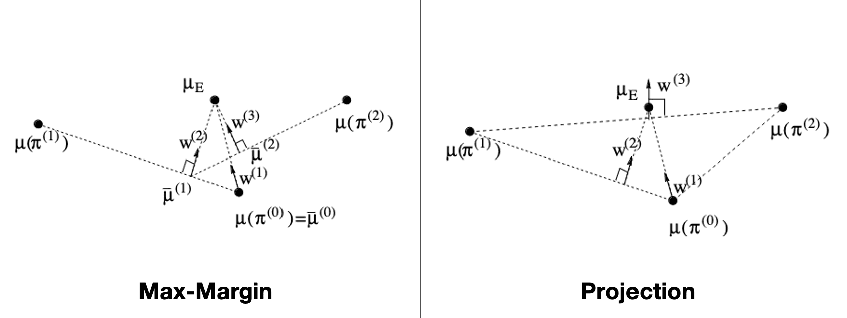
Max-Margin algorithm
The first is max-margin optimization that requires $K$-candidates \(\{ \pi^{(k)} \}_{k=1}^K\) of the best policy, which is consistent with previous IRL algorithms that the reward function should greatly distinguish the best and second best policy:
\[\begin{aligned} & \begin{array}{rcl} \texttt{Max-Margin:} & \underset{t, \boldsymbol{\alpha}}{\max} & \quad t \\ & \text { s.t. } & \boldsymbol{\alpha} \cdot \boldsymbol{\mu} (\pi^*) \geq \boldsymbol{\alpha} \cdot \boldsymbol{\mu} (\pi^{(k)}) + t, k = 1, \ldots, K \textrm{ and } \Vert \boldsymbol{\alpha} \Vert_2 \leq 1 \\ \\ \Longleftrightarrow & \max & \left\{ t = \underset{k = 1, \cdots, K}{\min} \boldsymbol{\alpha} \cdot \left( \boldsymbol{\mu} (\pi^*) - \boldsymbol{\mu} (\pi^{(k)}) \right) \right\} \\ & \text { s.t. } & \Vert \boldsymbol{\alpha} \Vert_2 \leq 1 \end{array} \end{aligned}\]Then, if $t \leq \varepsilon$ where $\varepsilon$ is a pre-defined threshold, then we find a new policy $\pi^{(K + 1)}$ that maximize the value function under the new reward function and add it into the candidate set.
Projection algorithm
Alternatively, if we do not wish to ask for human help to select a policy, we can automatically find the point closest to \(\pi^*\) in the convex closure of the feature expectations \(\{ \boldsymbol{\mu} (\pi^{(k)}) \}_{k=1}^K\) by solving the following quadratic programming, called projection formulation:
\[\begin{array}{ccl} \texttt{Projection: } & \min & \Vert \boldsymbol{\mu} (\pi^*) - \tilde{\boldsymbol{\mu}} \Vert_2 \\ & \text { s.t. } & \tilde{\boldsymbol{\mu}} = \sum_{k = 1}^K \lambda_k \boldsymbol{\mu} (\pi^{(k)}) \textrm{ where } \lambda_i \geq 0 \textrm{ and } \sum_{k = 1}^K \lambda_k = 1 \end{array}\]The following figure illustrates the geometric description of these policy iterations:
Maximum Margin Planning (MMP)
Ratliff et al. ICML 2006 proposed a quadratic programming formulation called maximum margin planning (MMP) where the objective is to find a linear mapping of feature expectations $\boldsymbol{\alpha} \cdot \boldsymbol{\mu} (\pi)$ to rewards $R$ so that the policy estimated from the reward function is close to the behavior in the demonstrations. With the optimal policy \(\pi^*\), MMP stems from the standard max-margin formulation of feature expectations \(\Vert \boldsymbol{\mu} (\pi^*) - \boldsymbol{\mu} (\pi) \Vert_2\):
\[\begin{array}{cl} \underset{\boldsymbol{\alpha}}{\min} & \dfrac{1}{2} \Vert \boldsymbol{\alpha} \Vert_2^2 \\ \text { s.t. } & \boldsymbol{\alpha} \cdot \boldsymbol{\mu} (\pi^*) \geq \boldsymbol{\alpha} \cdot \boldsymbol{\mu} (\pi) + 1 \quad \forall \pi \in \{ \pi_0, \pi_1, \cdots \} \end{array}\]Note that this optimization yields $\boldsymbol{\alpha}$ such that the expert policy \(\pi^*\) maximally outperforms the policies in the set \(\{ \pi_0, \pi_1, \cdots \}\) since minimizing $\Vert \boldsymbol{\alpha} \Vert_2$ is equivalent to maximize the margin of feature expectations:
\[\Vert \boldsymbol{\mu} (\pi^*) - \boldsymbol{\mu} (\pi) \Vert_2 \geq \frac{1}{\Vert \boldsymbol{\alpha} \Vert_2}\]by the constraints in the problem. The authors improved this formulation by incorporating:
- Similarity function $m (\pi^*, \pi)$
To give larger margin for policies that are very distinct from $\pi^*$, they incorporated the similarity function $m(\pi^*, \pi)$ that quantifies how dissimilar two policies are: $$ \begin{array}{cl} \underset{\boldsymbol{\alpha}}{\min} & \dfrac{1}{2} \Vert \boldsymbol{\alpha} \Vert_2^2 \\ \text { s.t. } & \boldsymbol{\alpha} \cdot \boldsymbol{\mu} (\pi^*) \geq \boldsymbol{\alpha} \cdot \boldsymbol{\mu} (\pi) + m (\pi^*, \pi) \quad \forall \pi \in \{ \pi_0, \pi_1, \cdots \} \end{array} $$ For example, we can set $m$ to return the number of states that $\pi$ visits that $\pi^*$ did not. - Slack variable $\xi$
Similar to soft margin SVM, they incorporated the additional slack variable $\xi$ to compensate some noises from the sub-optimality of expert $\pi^*$: $$ \begin{array}{cl} \underset{\boldsymbol{\alpha}}{\min} & \dfrac{1}{2} \Vert \boldsymbol{\alpha} \Vert_2^2 + C \xi \\ \text { s.t. } & \boldsymbol{\alpha} \cdot \boldsymbol{\mu} (\pi^*) \geq \boldsymbol{\alpha} \cdot \boldsymbol{\mu} (\pi) + m (\pi^*, \pi) - \xi \quad \forall \pi \in \{ \pi_0, \pi_1, \cdots \} \end{array} $$ where $C > 0$ is a hyperparameter that is used to penalize the amount of assumed sub-optimality.
Although the problem has very large number of constraints, the authors constructed the efficient algorithm with subgradient method. Please refer to the original paper for more implementation details.
Bayesian IRL (BIRL)
As previously noted, the IRL problem is ill-posed due to the inherent uncertainty in the reward function obtained. Consequently, it is natural to employ a probability distribution to model this uncertainty. Bayesian IRL addresses the problem from this perspective, treating the demonstration sequences as the likelihood. The foundational concept of Bayesian IRL was first introduced by Ramachandran et al., ICJAI 2007.
Let \(\tau = \{ (\mathbf{s}_0, \mathbf{a}_0), (\mathbf{s}_1, \mathbf{a}_1), \cdots, (\mathbf{s}_T, \mathbf{a}_T) \}\) represent one of the expert’s demonstrations. Bayesian IRL basically posits that the expert \(\pi^*\) behaves greedily, always selecting actions with the highest Q-value according to reward function $R$. This assumption results in the policy to be stationary, in other words, \(\pi^*\) is invariant with regard to time $t$ and does not change depending on \(\mathbf{a}_{1:t-1}\) and \(\mathbf{s}_{1:t-1}\) made in previous time steps. This assumption of independence yields the following factorization of the likelihood:
\[p (\tau \vert \mathbf{R}) = \prod_{t = 0}^T p \left( (\mathbf{s}_t, \mathbf{a}_t) \vert \mathbf{R} \right)\]Then, with a prior distribution $p(\mathbf{R})$ over the reward functions, we can compute the posterior distribution of the reward function $\mathbf{R}$ by Bayes theorem:
\[p (\mathbf{R} \vert \tau) \propto p (\tau \vert \mathbf{R}) \cdot p (\mathbf{R})\]Consequently, such probabilistic formulation has several advantages:
-
(1) It relies solely on demonstrations rather than requiring the optimal policy itself.
-
(2) It does not assume that the expert’s decision-making is flawless.
-
(3) External information about the problem can be integrated into the reward function through the prior distribution.
Original BIRL Algorithm
The expert’s objective of maximizing accumulated reward is equivalent to selecting the action that maximizes the Q-value $Q^{\pi^*}$ at each state. Building on this intuition, the original algorithm of Ramachandran et al., ICJAI 2007 models the likelihood of $(\mathbf{s}, \mathbf{a})$ as a Boltzmann distribution with the Q-value \(Q^{\pi^*}\) of an optimal policy \(\pi^*\):
\[p \left( (\mathbf{s}, \mathbf{a}) \vert \mathbf{R} \right) \propto \exp \left( \frac{Q^{\pi^*} (\mathbf{s}, \mathbf{a} ; \mathbf{R})}{\beta} \right)\]where $\beta$ is a parameter representing the confidence in the optimality of the expert \(\pi^*\). Consequently, by defining the summation of Q-values $E$ of the entire episode:
\[E (\tau, \mathbf{R}) = \sum_{t=0}^{T-1} Q^{\pi^*} (\mathbf{s}_t, \mathbf{a}_t ; \mathbf{R})\]the posterior probability is given by:
\[p (\mathbf{R} \vert \tau) = \frac{1}{Z} \exp \left( \frac{E (\tau, \mathbf{R})}{\beta} \right) \cdot p (\mathbf{R})\]where $Z$ is the normalizing factor that can be solved through sampling algorithms. The authors suggests several different priors over the continuous space of reward functions:
- Uniform prior
For an agnostic choice, we can use the uniform distribution: $$ p (\mathbf{R} (\mathbf{s}) = r) = \frac{1}{R_{\max} - R_{\min}} \quad \forall \mathbf{s} \in \mathcal{S} $$ - Gaussian or Laplacian prior
In several real-world MDPs with a sparse reward structure, where most states have negligible rewards, a Gaussian or Laplacian prior is more appropriate: $$ \begin{aligned} \texttt{Gaussian:} & \; p (\mathbf{R} (\mathbf{s}) = r) = \frac{1}{\sqrt{2\pi} \sigma} \exp \left( - \frac{r^2}{2 \sigma^2} \right) \quad \forall \mathbf{s} \in \mathcal{S} \\ \texttt{Laplacian:} & \; p (\mathbf{R} (\mathbf{s}) = r) = \frac{1}{2 \sigma} \exp \left( - \frac{\vert r \vert}{2 \sigma} \right) \quad \forall \mathbf{s} \in \mathcal{S} \\ \end{aligned} $$ - Beta prior
If the MDP reflects a planning-type problem with a significant dichotomy in rewards-where goal states exhibiting a large positive reward-a Beta distribution might be better suited: $$ p (\mathbf{R} (\mathbf{s}) = r) = \frac{1}{\sqrt{\frac{r}{R_{\max}}} \cdot \sqrt{1 - \frac{r}{R_{\max}}} } \quad \forall \mathbf{s} \in \mathcal{S} $$
Approximate Variational Reward Imitation Learning (AVRIL)
Following Ramachandran et al., 2007, various studies attempted to advance the foundational framework of BIRL by incorporating techniques such as Gaussian distribution, MAP inference, and multiple rewards. These methods involve sampling a new reward and evaluating the likelihood $p(\mathcal{D} \vert \mathbf{R})$ at each iteration, requiring the calculation of the Q-values \(Q^{\pi^*}\) with respect to $\mathbf{R}$ — in other words, performing forward RL. Consequently, they typically do not scale efficiently to large and modern environments and often necessitate substantial interaction with the environment.
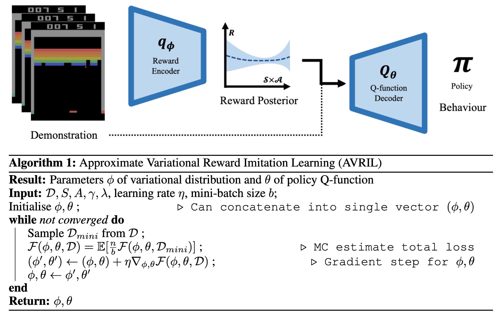
Recently, Chan et al., 2021 addressed these challenges by simultaneously learning an approximate reward posterior distribution that scales to arbitrarily complicated state spaces alongside an appropriate policy in a completely offline manner through a variational approach. This method is aptly named approximate variational reward imitation learning (AVRIL).
Algorithm
Let \(\mathcal{D} = \{ \tau_i \}_{i=1}^N\) be the dataset of the expert’s demonstrations. Traditionally, BIRL approaches have predominantly utilized sampling or MAP-based methods for inferring the posterior $p ( \mathbf{R} \vert \mathcal{D} )$. In contrast, AVRIL reformulates the BIRL problem as variational inference, employing surrogate distribution $q_\phi (R)$:
\[\underset{\phi}{\min} \; \left\{ \mathrm{KL} \left( q_\phi (\mathbf{R}) \Vert p (\mathbf{R} \vert \mathcal{D} ) \right) \right\}\]To avoid the intractability, this objective is rewritten into an auxiliary Evidence Lower Bound (ELBO) objective:
\[\mathcal{L}_{\texttt{ELBO}} (\phi) = \mathbb{E}_{q_\phi} \left[ \log p (\mathcal{D} \vert \mathbf{R}) \right] - \mathrm{KL} \left( q_\phi (\mathbf{R}) \Vert p (R) \right)\]Assuming the Boltzmann distribution for the likelihood $p(\mathcal{D} \vert R)$, we obtain:
\[\mathcal{L}_{\texttt{ELBO}} (\phi) = \mathbb{E}_{q_\phi} \left[ \sum_{(\mathbf{s}, \mathbf{a}) \in \mathcal{D}} \log \frac{\exp (Q^{\pi^*} (\mathbf{s}, \mathbf{a} ; \mathbf{R}) / \beta)}{\sum_{\mathbf{a}^\prime \in \mathcal{A}} \exp (Q^{\pi^*} (\mathbf{s}, \mathbf{a}^\prime ; \mathbf{R}) / \beta)} \right] - \mathrm{KL} \left( q_\phi (\mathbf{R}) \Vert p (\mathbf{R}) \right)\]Additionally, AVRIL employs a second neural network $Q_\theta$ to learn \(Q^{\pi^*}\). It is important to note that a standard Q-function, which represents the entire distribution, cannot be learned directly due to the constraints of each individual state-action pair:
\[\mathbf{R} (\mathbf{s}, \mathbf{a}) = \mathbb{E}_{\mathbf{s}^\prime \sim \mathbb{P}_\mathcal{S} (\cdot \vert \mathbf{s}, \mathbf{a}), \mathbf{a}^\prime \sim \pi (\cdot \vert \mathbf{s}^\prime)} \left[Q^\pi (\mathbf{s}, \mathbf{a}; \mathbf{R}) - \gamma Q^\pi (\mathbf{s}^\prime, \mathbf{a}^\prime; \mathbf{R}) \right]\]To ensure consistency between the reward $\mathbf{R}$ ($q_\phi$) and the Q-values $Q_\theta$, AVRIL imposes a constraint that the implied reward of the policy is sufficiently probable under the variational posterior (equivalently, that the negative log-likelihood is sufficiently low):
\[\begin{array}{cl} \underset{\phi, \theta}{\max} & \sum_{(\mathbf{s}, \mathbf{a}) \in \mathcal{D}} \log \frac{\exp (Q_\theta (\mathbf{s}, \mathbf{a}) / \beta)}{\sum_{\mathbf{a}^\prime \in \mathcal{A}} \exp (Q_\theta (\mathbf{s}, \mathbf{a}^\prime) / \beta)} - \mathrm{KL} \left( q_\phi (\mathbf{R}) \Vert p (\mathbf{R}) \right) \\ \text { s.t. } & \mathbb{E}_{\pi} \left[ - \log q_\phi \left( Q_\theta (\mathbf{s}, \mathbf{a}) - \gamma Q_\theta (\mathbf{s}^\prime, \mathbf{a}^\prime) \right) \right] < \varepsilon \end{array}\]which is equivalent to
\[\begin{aligned} \mathcal{L}_{\texttt{AVRIL}} (\phi, \theta, \mathcal{D}) = \sum_{(\mathbf{s}, \mathbf{a}, \mathbf{s}^\prime, \mathbf{a}^\prime) \in \mathcal{D}} & \log \frac{\exp \left( Q_\theta(\mathbf{s}, \mathbf{a}) / \beta \right)}{\sum_{\mathbf{b} \in \mathcal{A}}\exp( Q_\theta( \mathbf{s}, \mathbf{b}) / \beta)} - \mathrm{KL}\left(q_\phi(\mathbf{R}(\mathbf{s}, \mathbf{a})) \Vert p(\mathbf{R}(\mathbf{s}, \mathbf{a}))\right) \nonumber \\ & + \lambda \log q_\phi(Q_\theta(\mathbf{s}, \mathbf{a}) - \gamma Q_\theta( \mathbf{s}^\prime, \mathbf{a}^\prime)). \end{aligned}\]by Lagrangian under the KKT conditions.
Maximum Entropy (Max-Ent) IRL
IRL is intrinsically an ill-posed problem, as multiple reward functions can account for the expert’s behavior. And the presence of degenerate and multiple solutions led early approaches, such as apprenticeship learning (AIRP), to exhibit a side effect. Specifically, the feature expectation matching:
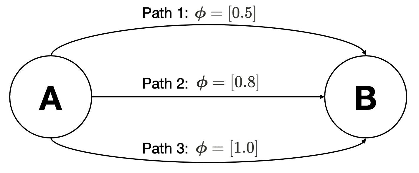
\[\boldsymbol{\mu} (\pi) = \mathbb{E}_{\pi} \left[ \sum_{t=0}^{T-1} \gamma^t \boldsymbol{\phi}(\mathbf{s}_t, \mathbf{a}_t) \right] = \boldsymbol{\mu} (\pi^*) = \mathbb{E}_{\pi^*} \left[ \sum_{t=0}^{T-1} \gamma^t \boldsymbol{\phi}(\mathbf{s}_t, \mathbf{a}_t) \right] \\\]is inadequate to ensure that \(\pi = \pi^*\), potentially causing the algorithm to malfunction; for example, it might assign zero probability to some of the demonstrated actions. In the following simple example with three demonstrated paths, suppose we determine an optimal reward weight $\boldsymbol{\alpha}$ by maximizing the feature expectation margin. There are then two non-degenerate optimal policies:
- $\pi_1$: if $\boldsymbol{\alpha} < 0$, path 1 should be selected;
- $\pi_2$: if $\boldsymbol{\alpha} > 0$, path 3 should be selected;
In this scenario, although the convex combination of feature expectations $\tilde{\boldsymbol{\mu}} = \lambda_1 \boldsymbol{\mu}(\pi_1) + \lambda_2 \boldsymbol{\mu}(\pi_2)$ obtained from the projection algorithm matches \(\boldsymbol{\mu} (\pi^*)\), the resulting convex mixture of policy $\lambda_1 \pi_1 + \lambda_2 \pi_2$ may not be optimal, as it never selects path 2, despite it being demonstrated by the expert.
Similar to the idea of BIRL, maximum entropy (Max-Ent) IRL adopts a probability approach to resolve the ill-posed problem of the original IRL. The key idea in the maximum entropy approaches is to not only match the feature expectations, but also remove ambiguity in the path distribution $p (\tau \vert \mathbf{R})$ by trying to make $p (\tau \vert \mathbf{R})$ as being no more committed to any particular path as possible.
\[\begin{aligned} p^* (\tau \vert \mathbf{R}) & = \underset{p}{\arg \max} \; \mathbb{H} (p) \\ & = \begin{aligned}[t] & \underset{p}{\arg \max} \; \int - p (\tau \vert \mathbf{R}) \log p (\tau \vert \mathbf{R}) \; d \tau \\ & \text{ s.t. } \begin{aligned}[t] & \mathbb{E}_{\tau \sim p (\tau \vert \mathbf{R})} \left[ \sum_{t=0}^{T-1} \gamma^t \boldsymbol{\phi}(\mathbf{s}_t, \mathbf{a}_t) \right] = \boldsymbol{\mu} (\pi^*) = \mathbb{E}_{\pi^*} \left[ \sum_{t=0}^{T-1} \gamma^t \boldsymbol{\phi}(\mathbf{s}_t, \mathbf{a}_t) \right] \\ & \int p (\tau \vert \mathbf{R}) d \tau = 1 \text{ and } p (\tau \vert \mathbf{R}) \geq 0 \; \forall \tau \in \mathcal{D} \end{aligned} \end{aligned} \end{aligned}\]Original Max-Ent IRL Algorithm
Ziebart et al. AAAI 2008 proposed the first Max-Ent IRL algorithm that utilized feature expectation matching and similar probabilistic model with the first BIRL algorithm:
\[p \left( \mathbf{a} \vert \mathbf{s}, \mathbf{R} \right) \propto \exp \left( \frac{Q^{\pi^*} (\mathbf{s}, \mathbf{a} ; \mathbf{R})}{\beta} \right)\]where \(Q^{\pi^*} (\mathbf{s}, \mathbf{a} ; \mathbf{R})\) is estimated by a linear combination of features $\boldsymbol{\phi} (\mathbf{s}, \mathbf{a})$ with respect to the reward weight $\boldsymbol{\theta}$:
\[\begin{aligned} \mathbf{R}(\mathbf{s}, \mathbf{a}) & = \boldsymbol{\theta} \cdot \boldsymbol{\phi} (\mathbf{s}, \mathbf{a} = \pi^* (\mathbf{s})) \\ Q^{\pi^*} (\mathbf{s}, \mathbf{a}) & = \mathbb{E}_{\pi^*} \left[ \sum_{t=0}^\infty \gamma^t \mathbf{R}(\mathbf{s}, \mathbf{a}) \right] = \boldsymbol{\theta} \cdot \mathbb{E}_{\pi^*} \left[ \sum_{t=0}^\infty \gamma^t \boldsymbol{\phi} (\mathbf{s}, \mathbf{a}) \right] \equiv \boldsymbol{\theta} \cdot \mathbf{f}(\mathbf{s}, \mathbf{a}) \end{aligned}\]where $\mathbf{f}(\mathbf{s}, \mathbf{a})$ is the feature expectation. This gives:
\[\begin{aligned} & \; p(\tau \vert \mathbf{R}) = \frac{1}{Z (\boldsymbol{\theta})} \exp \left( \frac{\boldsymbol{\theta} \cdot \mathbf{f} (\tau)}{\beta} \right) \cdot \mu (\mathbf{s}_0) \prod_{t=0} \mathbb{P}_\mathcal{S} (\mathbf{s}_{t+1} \vert \mathbf{s}_t, \mathbf{a}_t) \equiv \frac{1}{Z (\boldsymbol{\theta})} \exp \left( \frac{\boldsymbol{\theta} \cdot \mathbf{f} (\tau)}{\beta} \right) \cdot p (\tau) \\ & \text{ where } \begin{aligned}[t] \mathbf{f} (\tau) & = \sum_{t=0}^T \mathbf{f} (\mathbf{s}_t, \mathbf{a}_t) \\ Z (\boldsymbol{\theta}) & = \int \exp \left( \frac{\boldsymbol{\theta} \cdot \mathbf{f} (\tau)}{\beta} \right) \cdot p (\tau) d \tau \end{aligned} \end{aligned}\]From the optimization theory, it is known that maximum likelihood estimation (MLE) in exponential (Gibbs) family models is equivalent to maximum entropy optimization under some constraints:
Let $\mathcal{D} = \{ \mathbf{x}_i \}_{i=1}^N$ be the dataset of $N$ i.i.d. observations. The optimal solution $p^*$ of the following maximum entropy problem with some constraint functions $\boldsymbol{\phi}$: $$ \begin{aligned} & p^* = \underset{p \in \mathcal{P}}{\arg \max} \; \mathbb{H}(p) \\ & \text{ s.t. } \; \mathbb{E}_{\mathbf{x} \sim p} \left[ \phi_d (\mathbf{x}) \right] = \frac{1}{N} \sum_{i=1}^N \phi_d (\mathbf{x}_i) \quad \forall d = 1, \dots, D \end{aligned} $$ is of the form: $$ p^* (\mathbf{x}) \propto \exp \left( \boldsymbol{\theta} \cdot \boldsymbol{\phi} (\mathbf{s}) \right) $$ where $\boldsymbol{\theta}$ are chosen to satisfy the constraints.
Conversely, the maximum likelihood solution of $p_\boldsymbol{\theta}$ of the form: $$ p_\boldsymbol{\theta} (\mathbf{x}) \propto \exp \left( \boldsymbol{\theta} \cdot \boldsymbol{\phi} (\mathbf{s}) \right) $$ satisfies the constraints of the above maximum entropy problem. In other words, the maximum likelihood solution is the optimal solution of the maximum entropy problem.
$\mathbf{Proof.}$
Max-Ent $\implies$ MLE
By introducing Lagrange multipliers $\boldsymbol{\theta}$ and $\eta_0$, we discard the constraint of the maximum entropy problem; consider the follwowing functional:
\[\mathcal{L} (p)= \in _{-\infty}^{\infty} p(x) \log {p(\mathbf{x})} d\mathbf{x} - \eta_{0}\left(\int_{-\infty}^{\infty}p(\mathbf{x})d\mathbf{x} - 1\right)-\sum_{j=1}^{D}\theta_{j}\left(\int_{-\infty}^{\infty} \phi_{j}(\mathbf{x})p(\mathbf{x})d \mathbf{x}- \hat{\mu}_j \right)\]where
\[\hat{\mu}_j = \frac{1}{N} \sum_{i=1}^N \phi_j (\mathbf{x}_i).\]By setting the derivative to be zero:
\[\frac{\partial J}{\partial p} = \log p(\mathbf{x}) + 1 - \eta_0 - \boldsymbol{\theta} \cdot \boldsymbol{\phi} (\mathbf{x}) = 0\]Therefore, the optimal distribution $p^*$ must be the form of:
\[p(\mathbf{x}) = e^{- 1 + \eta_0} \cdot e^{\boldsymbol{\theta} \cdot \boldsymbol{\phi} (\mathbf{x})}\]which proves the first statement.
MLE $\implies$ Max-Ent
The log-likelihood of $p_\boldsymbol{\theta}$ is given by:
\[\mathcal{L}(\boldsymbol{\theta}; \mathcal{D}) = \sum_{i=1}^N \log p_\boldsymbol{\theta} (\mathbf{x}_i) = \sum_{i=1}^N \boldsymbol{\theta} \cdot \boldsymbol{\phi} (\mathbf{x}_i) - N \cdot Z (\theta)\]where $Z(\theta)$ is the log-partition function:
\[Z(\theta) = \log \left( \int \exp \left( \boldsymbol{\theta} \cdot \boldsymbol{\phi} (\mathbf{x}) \right) d \mathbf{x} \right)\]By setting $\nabla_\boldsymbol{\theta} \mathcal{L} (\boldsymbol{\theta} ; \mathcal{D})$, we obtain the equation of the MLE of $\boldsymbol{\theta}$:
\[\nabla_{\boldsymbol{\theta}} Z (\theta) = \frac{1}{N} \sum_{i=1}^N \boldsymbol{\phi} (\mathbf{x}_i)\]Noting that:
\[\nabla_{\boldsymbol{\theta}} Z (\theta) = \mathbb{E}_{\mathbf{x} \sim p_\boldsymbol{\theta}} \left[ \boldsymbol{\phi} (\mathbf{x}) \right]\]we proved the theorem.
\[\tag*{$\blacksquare$}\]Therefore, approximating \(\boldsymbol{\mu} (\pi^*)\) with the Monte Carlo estimator, the parameter $\boldsymbol{\theta}$ can be optimized by maximizing the log-likelihood of $p(\tau \vert \mathbf{R})$:
\[\mathcal{L}_{\texttt{Max-Ent}} (\boldsymbol{\theta}) = \frac{1}{N} \sum_{i=1}^N \log p (\tau_i \vert \mathbf{R}) = \frac{1}{N} \sum_{i=1}^N \frac{\boldsymbol{\theta} \cdot \mathbf{f} (\tau_i)}{\beta} - \log Z (\boldsymbol{\theta})\]Note that $p(\tau)$ is ignored as it is independent of $\boldsymbol{\theta}$. The authors adopted gradient ascent for the optimization where the gradient of loss is given by:
\[\begin{aligned} \nabla_{\boldsymbol{\theta}} \mathcal{L}_{\texttt{Max-Ent}} (\boldsymbol{\theta}) & = \frac{1}{N} \sum_{i=1}^N \frac{\mathbf{f}(\tau_i)}{\beta} - \frac{1}{Z (\boldsymbol{\theta})} \int p(\tau) \cdot \exp \left( \frac{\boldsymbol{\theta} \cdot \mathbf{f} (\tau)}{\beta} \right) \frac{\mathbf{f} (\tau)}{\beta} d \tau \\ & = \frac{1}{N} \sum_{i=1}^N \frac{\mathbf{f}(\tau_i)}{\beta} - \mathbb{E}_{\tau \sim p(\tau \vert \mathbf{R})} \left[ \frac{\mathbf{f} (\tau)}{\beta} \right] \\ & \propto \underbrace{\frac{1}{N} \sum_{i=1}^N \mathbf{f}(\tau_i)}_{\text{estimate with expert sample}} - \underbrace{\mathbb{E}_{\tau \sim p(\tau \vert \mathbf{R})} \left[ \mathbf{f}(\tau) \right]}_{\text{soft optimal policy under current reward } \mathbf{R}} \\ & = \frac{1}{N} \sum_{i=1}^N \sum_{t=0}^T \mathbf{f}(\mathbf{s}_t^i, \mathbf{a}_t^i) - \sum_{t=0}^T \mathbb{E}_{\mathbf{s}_t \sim p(\mathbf{s}_t \vert \mathbf{R}), \mathbf{a}_t \sim p (\mathbf{a}_t \vert \mathbf{s}_t, \mathbf{R})} \left[ \mathbf{f}(\mathbf{s}_t, \mathbf{a}_t) \right] \\ & = \frac{1}{N} \sum_{i=1}^N \sum_{t=0}^T \mathbf{f}(\mathbf{s}_t^i, \mathbf{a}_t^i) - \sum_{t=0}^T \int_\mathcal{A} \int_\mathcal{S} \rho_t (\mathbf{s}_t, \mathbf{a}_t) \mathbf{f}(\mathbf{s}_t, \mathbf{a}_t) d \mathbf{s}_t d \mathbf{a}_t \end{aligned}\]where $\rho_t (\mathbf{s}, \mathbf{a})$ is a state-action visitation probability of $(\mathbf{s}, \mathbf{a})$ at time step $t$. Since we typically assume that the transition probability is known in IRL problems, the authors estimated the second term through Monte Carlo sampling.
Maximum Causal Entropy (MCE) IRL
In stochastic MDP (i.e., \(\mathbb{P}_\mathcal{S} (\mathbf{s}^\prime \vert \mathbf{s}, \mathbf{a}) > 0\)), the original Max-Ent IRL calculates the entropy over the entire trajectory distribution, incorporating an undesirable dependence on transition dynamics through terms $\mathbb{H} (\mathbb{P}_\mathcal{S})$:
\[\begin{aligned} \mathbb{H} \left( p ( \mathbf{s}_{0:T-1}, \mathbf{a}_{0:T-1}, \vert \mathbf{R}) \right) & =\sum_{t=0}^{T-1} \mathbb{H} \left( p (\mathbf{s}_t, \mathbf{a}_t \mid \mathbf{s}_{0: t-1}, \mathbf{a}_{0: t-1}) \right) & \because \textrm{ chain rule } \\ & =\sum_{t=0}^{T-1} \mathbb{H} \left( p (\mathbf{s}_t \mid \mathbf{s}_{0: t-1}, \mathbf{a}_{0: t-1}) \right)+\sum_{t=0}^{T-1} \mathbb{H} \left( p( \mathbf{a}_t \mid \mathbf{s}_{0: t}, \mathbf{a}_{0: t-1}) \right) & \because \textrm{ chain rule } \\ & =\sum_{t=0}^{T-1} \mathbb{H} \left( p (\mathbf{s}_t \mid \mathbf{s}_{t-1}, \mathbf{a}_{t-1}) \right)+\sum_{t=0}^{T-1} \mathbb{H} \left( p (\mathbf{a}_t \mid \mathbf{s}_t ) \right) & \because \text{ Markov property } \\ & =\sum_{t=0}^{T-1} \underbrace{\mathbb{H} \left( \mathbb{P}_\mathcal{S} \right)}_{\text {state transition entropy}}+\underbrace{\mathbb{H} \left( \mathbf{a}_{0: T-1} \Vert \mathbf{s}_{0: T-1}\right)}_{\text {causal entropy }} \end{aligned}\]Maximizing Shannon entropy therefore introduces a bias towards selecting actions with uncertain, and possibly risky, outcomes. Consequently, maximum causal entropy (MCE) IRL is to be favored over maximum Shannon entropy IRL in stochastic MDPs. It is important to noting that MCE IRL reduces into the original Max-Ent IRL for deterministic MDP cases.
Causal entropy: $$ \mathbb{H} (\mathbf{a}^T \Vert \mathbf{s}^T) \equiv \mathbb{E}_\pi \left[ - \log p (\mathbf{a}^T \Vert \mathbf{s}^T) \right] = \sum_{t=0}^{T-1} \mathbb{H}(\mathbf{a}_t \vert \mathbf{s}_{1:t}, \mathbf{a}_{1:t-1}) $$ measures the uncertainty present in the causally conditioned distribution: $$ p(\mathbf{a}^T \vert \mathbf{s}^T) \equiv \prod_{t=1}^{T-1} p (\mathbf{a}_t \vert \mathbf{s}_{1:t}, \mathbf{a}_{1:t-1}) = \prod_{t=1}^{T-1} \pi (\mathbf{a}_t \vert \mathbf{s}_t) \; \text{on MDP} $$
Consequently, the MCE IRL problem can be formulated as:
\[\begin{aligned} \texttt{MCE IRL: } p^* (\mathbf{a}_t \vert \mathbf{s}_{1:t}, \mathbf{a}_{1:t-1}) & = \underset{p}{\arg \max} \; \mathbb{H} (\mathbf{a}^T \Vert \mathbf{s}^T) \\ & \text{ s.t. } \begin{aligned}[t] & \mathbb{E}_{\mathbf{s}_{t + 1} \sim \mathbb{P}_\mathcal{S} (\cdot \vert \mathbf{s}_t, \mathbf{a}_t), \mathbf{a}_t \sim p (\cdot \vert \mathbf{s}_{1:t}, \mathbf{a}_{1:t-1})} \left[ \sum_{t=0}^{T-1} \gamma^t \boldsymbol{\phi}(\mathbf{s}_t, \mathbf{a}_t) \right] = \boldsymbol{\mu} (\pi^*) = \mathbb{E}_{\pi^*} \left[ \sum_{t=0}^{T-1} \gamma^t \boldsymbol{\phi}(\mathbf{s}_t, \mathbf{a}_t) \right] \\ & \int p (\mathbf{a}_t \vert \mathbf{s}_{1:t}, \mathbf{a}_{1:t-1}) d \mathbf{a}_t = 1 \text{ and } p (\mathbf{a}_t \vert \mathbf{s}_{1:t}, \mathbf{a}_{1:t-1}) \geq 0 \; \forall \tau \in \mathcal{D} \end{aligned} \end{aligned}\]Note that under the MDP environment, \(p^* (\mathbf{a}_t \vert \mathbf{s}_{1:t}, \mathbf{a}_{1:t-1})\) can be replaced by \(p^* (\mathbf{a}_t \vert \mathbf{s}_t)\). Introducing the Lagrangian multipliers $\boldsymbol{\theta}$ and deriving the dual problem, we have the following auxiliary loss:
\[\begin{aligned} \mathcal{L}(\boldsymbol{\theta}) = & \; \underset{\pi}{\max} \Bigl\{ \mathbb{H} (\mathbf{a}^T \Vert \mathbf{s}^T) \\ & \; + \boldsymbol{\theta} \cdot \left( \mathbb{E}_{\mathbf{s}_{t + 1} \sim \mathbb{P}_\mathcal{S} (\cdot \vert \mathbf{s}_t, \mathbf{a}_t), \mathbf{a}_t \sim \pi_\boldsymbol{\theta} (\cdot \vert \mathbf{s}_t)} \left[ \sum_{t=0}^{T-1} \gamma^t \boldsymbol{\phi}(\mathbf{s}_t, \mathbf{a}_t) \right] - \mathbb{E}_{\pi^*} \left[ \sum_{t=0}^{T-1} \gamma^t \boldsymbol{\phi}(\mathbf{s}_t, \mathbf{a}_t) \right] \right) \Bigr\} \end{aligned}\]and can show that the optimal distribution has a form which resembles the optimal policy under soft value iteration:
The optimal distribution $p^*$ of the maximum causal entropy (MCE) constrained optimization under the MDP is defined by: $$ \pi_{\boldsymbol{\theta}} (\mathbf{a}_t \vert \mathbf{s}_t) = \exp \left( Q_{\boldsymbol{\theta}}^{\texttt{soft}} (\mathbf{s}_t, \mathbf{a}_t) - V_{\boldsymbol{\theta}}^{\texttt{soft}} (\mathbf{s}_t) \right) $$ where $V_{\boldsymbol{\theta}}^{\texttt{soft}}$ and $Q_{\boldsymbol{\theta}}^{\texttt{soft}}$ are defined recursively as: $$ \begin{aligned} V_{\boldsymbol{\theta}}^{\texttt{soft}} (\mathbf{s}_t) & = \log \sum_{\mathbf{a}_t \in \mathcal{A}} \exp Q_{\boldsymbol{\theta}}^{\texttt{soft}} (\mathbf{s}_t, \mathbf{a}_t) \\ Q_{\boldsymbol{\theta}}^{\texttt{soft}} (\mathbf{s}_t, \mathbf{a}_t) & = \boldsymbol{\theta} \cdot \boldsymbol{\phi} (\mathbf{s}_t, \mathbf{a}_t) + \gamma \underset{\mathbf{s}_{t+1} \sim \mathbb{P}_\mathcal{S} (\cdot \vert \mathbf{s}_t, \mathbf{a}_t)}{\mathbb{E}} \left[V_{\boldsymbol{\theta}}^{\texttt{soft}} (\mathbf{s}_{t+1}) \mid \mathbf{s}_t, \mathbf{a}_t \right] \\ Q_{\boldsymbol{\theta}}^{\texttt{soft}} (\mathbf{s}_{T-1}, \mathbf{a}_{T-1}) & = \boldsymbol{\theta} \cdot \boldsymbol{\phi} (\mathbf{s}_{T-1}, \mathbf{a}_{T-1}) \end{aligned} $$ for all $0 \leq t < T - 1$.
$\mathbf{Proof.}$
The full Lagrangian for the MCE optimization problem under the MDP environment is given by:
\[\Psi (\boldsymbol{\lambda}, \boldsymbol{\theta}) = \mathcal{L}(\boldsymbol{\theta}) + \sum_{\mathbf{s}_t \in \mathcal{S}, 0 \leq t < T} \lambda_{\mathbf{s}_t} \left( \sum_{\mathbf{a} \in \mathcal{A}} \pi (\mathbf{a} \vert \mathbf{s}_t) - 1 \right).\]where $\boldsymbol{\lambda}$ is another Lagrangian multiplier independent of $\boldsymbol{\theta}$. For brevity, write \(h (\mathbf{s}_t) = \sum_{\mathbf{a} \in \mathcal{A}} \pi (\mathbf{a} \vert \mathbf{s}_t) - 1\).
$\mathbf{Proof.}$
We can derive the resulting gradient term-by-term. Assuming the MDP environment, \(p (\mathbf{a}_t \vert \mathbf{s}_{1:t}, \mathbf{a}_{1:t-1})\) can be replaced by \(\pi (\mathbf{a}_t \vert \mathbf{s}_t)\)
Gradient of Normalization Term
\[\begin{aligned} \nabla_{\pi (\mathbf{a}_t \vert \mathbf{s}_t)} \sum_{\mathbf{s}_{t^\prime} \in \mathcal{S}, 0 \leq t^\prime < T} \lambda_{\mathbf{s}_{t^\prime}} h (\mathbf{s}_{t^\prime}) & = \nabla_{\pi (\mathbf{a}_t \vert \mathbf{s}_t)} \sum_{t^\prime = 0}^{T - 1} \sum_{\mathbf{s}_{t^\prime} \in \mathcal{S}} \lambda_{\mathbf{s}_{t^\prime}} \sum_{\mathbf{a} \in \mathcal{A}} \pi (\mathbf{a} \vert \mathbf{s}_{t^\prime}) - 1 \\ & = \lambda_{\mathbf{s}_t} \end{aligned}\]Gradient of Feature Matching Term
\[\begin{aligned} & \nabla_{\pi (\mathbf{a}_t \vert \mathbf{s}_t)} \boldsymbol{\theta} \cdot \left( \mathbb{E}_{\mathbf{s}_{t^\prime + 1} \sim \mathbb{P}_\mathcal{S} (\cdot \vert \mathbf{s}_{t^\prime}, \mathbf{a}_{t^\prime}), \mathbf{a}_{t^\prime} \sim \pi (\cdot \vert \mathbf{s}_t^\prime)} \left[ \sum_{t^\prime=0}^{T-1} \gamma^t \boldsymbol{\phi}(\mathbf{s}_{t^\prime}, \mathbf{a}_{t^\prime}) \right] - \mathbb{E}_{\pi^*} \left[ \sum_{t=0}^{T-1} \gamma^t \boldsymbol{\phi}(\mathbf{s}_{t^\prime}, \mathbf{a}_{t^\prime}) \right] \right) \\ = & \; \nabla_{\pi (\mathbf{a}_t \vert \mathbf{s}_t)} \boldsymbol{\theta} \cdot \mathbb{E}_{\mathbf{s}_{t^\prime + 1} \sim \mathbb{P}_\mathcal{S} (\cdot \vert \mathbf{s}_{t^\prime}, \mathbf{a}_{t^\prime}), \mathbf{a}_{t^\prime} \sim \pi (\cdot \vert \mathbf{s}_t^\prime)} \left[ \sum_{t^\prime=0}^{T-1} \gamma^{t^\prime} \boldsymbol{\phi}(\mathbf{s}_{t^\prime}, \mathbf{a}_{t^\prime}) \right] \\ = & \; \boldsymbol{\theta} \cdot \mathbb{E}_{\mathbf{s}_{t^\prime + 1} \sim \mathbb{P}_\mathcal{S} (\cdot \vert \mathbf{s}_{t^\prime}, \mathbf{a}_{t^\prime})} \left[ \nabla_{\pi (\mathbf{a}_t \vert \mathbf{s}_t)} \mathbb{E}_{\mathbf{a}_{t^\prime} \sim \pi (\cdot \vert \mathbf{s}_{t^\prime})} \left[ \sum_{t^\prime=0}^{T-1} \gamma^{t^\prime} \boldsymbol{\phi}(\mathbf{S}_{t^\prime}, \mathbf{A}_{t^\prime}) \middle\vert \mathbf{S}_t = \mathbf{s}_{t} \right] \right] \\ = & \; \boldsymbol{\theta} \cdot \mathbb{E}_{\mathbf{s}_{t^\prime + 1} \sim \mathbb{P}_\mathcal{S} (\cdot \vert \mathbf{s}_{t^\prime}, \mathbf{a}_{t^\prime})} \left[ \gamma^t \delta (\mathbf{S}_t = \mathbf{s}_t) \nabla_{\pi (\mathbf{a}_t \vert \mathbf{s}_t)} \mathbb{E}_{\mathbf{a}_t \sim \pi (\cdot \vert \mathbf{s}_t)} \left[ \sum_{t^\prime=t}^{T-1} \gamma^{t^\prime - t} \boldsymbol{\phi}(\mathbf{S}_{t^\prime}, \mathbf{A}_{t^\prime}) \middle\vert \mathbf{S}_t = \mathbf{s}_t \right] \right] \\ = & \; \rho_{\pi, t} (\mathbf{s}_t) \boldsymbol{\theta} \cdot \nabla_{\pi (\mathbf{a}_t \vert \mathbf{s}_t)} \mathbb{E}_{\mathbf{a}_t \sim \pi (\cdot \vert \mathbf{s}_t)} \left[ \sum_{t^\prime=t}^{T-1} \gamma^{t^\prime - t} \boldsymbol{\phi}(\mathbf{S}_{t^\prime}, \mathbf{A}_{t^\prime}) \middle\vert \mathbf{S}_t = \mathbf{s}_t \right] \\ = & \; \rho_{\pi, t} (\mathbf{s}_t) \boldsymbol{\theta} \cdot \nabla_{\pi (\mathbf{a}_t \vert \mathbf{s}_t)} \mathbb{E}_{\mathbf{a}_t \sim \pi (\cdot \vert \mathbf{s}_t)} \left[ \sum_{t^\prime=t}^{T-1} \gamma^{t^\prime - t} \boldsymbol{\phi}(\mathbf{S}_{t^\prime}, \mathbf{A}_{t^\prime}) \middle\vert \mathbf{S}_t = \mathbf{s}_t, \mathbf{A}_t = \mathbf{a}_t \right] \\ = & \; \rho_{\pi, t} (\mathbf{s}_t) \boldsymbol{\theta} \cdot \left[ \boldsymbol{\phi} (\mathbf{s}_t, \mathbf{a}_t) + \mathbb{E}_{\mathbf{a}_t \sim \pi (\cdot \vert \mathbf{s}_t)} \left[ \sum_{t^\prime=t+1}^{T-1} \gamma^{t^\prime - t} \boldsymbol{\phi}(\mathbf{S}_{t^\prime}, \mathbf{A}_{t^\prime}) \middle\vert \mathbf{S}_t = \mathbf{s}_t, \mathbf{A}_t = \mathbf{a}_t \right] \right] \end{aligned}\]Gradient of Causal Entropy Term
\[\begin{aligned} & \nabla_{\pi (\mathbf{a}_t \vert \mathbf{s}_t)} \mathbb{H}(\mathbf{a}^{T-1} \Vert \mathbf{s}^{T-1}) \\ = & \; - \nabla_{\pi (\mathbf{a}_t \vert \mathbf{s}_t)} \mathbb{E}_\pi \left[ - \sum_{t^\prime = 0}^{T-1} \log \pi (\mathbf{a}_{t^\prime} \vert \mathbf{s}_{t^\prime}) \right] \\ = & \; - \rho_{\pi, t} (\mathbf{s}_t) \nabla_{\pi (\mathbf{a}_t \vert \mathbf{s}_t)} \mathbb{E}_\pi \left[ \sum_{t^\prime = t}^{T-1} \log \pi (\mathbf{A}_{t^\prime} \vert \mathbf{S}_{t^\prime}) \middle\vert \mathbf{S}_t = \mathbf{s}_t \right] \\ = & \; - \rho_{\pi, t} (\mathbf{s}_t) \nabla_{\pi (\mathbf{a}_t \vert \mathbf{s}_t)} \mathbb{E}_\pi \left[ \log \pi (\mathbf{A}_t \vert \mathbf{S}_t) + \sum_{t^\prime = t + 1}^{T-1} \log \pi (\mathbf{A}_{t^\prime} \vert \mathbf{S}_{t^\prime}) \middle\vert \mathbf{S}_t = \mathbf{s}_t \right] \\ = & \; - \rho_{\pi, t} (\mathbf{s}_t) \left[ 1 + \log \pi (\mathbf{a}_t \vert \mathbf{s}_t) + \mathbb{E}_\pi \left[ \sum_{t^\prime = t + 1}^{T-1} \log \pi (\mathbf{A}_{t^\prime} \vert \mathbf{S}_{t^\prime}) \middle\vert \mathbf{S}_t = \mathbf{s}_t \right] \right] \\ \end{aligned}\] \[\tag*{$\blacksquare$}\]By setting the gradient to be zero and re-arranging terms, we have:
\[\begin{aligned} \pi (\mathbf{a}_t \vert \mathbf{s}_t) = & \exp \Biggl( \boldsymbol{\theta} \cdot \boldsymbol{\phi} (\mathbf{s}_t, \mathbf{a}_t) - 1 + \frac{\lambda_{\mathbf{s}_t}}{\rho_{\pi, t} (\mathbf{s}_t)}\\ + \mathbb{E}_\po\i \left[ \sum_{t^\prime = t + 1}^{T - 1} \gamma^{t^\prime - t} \boldsymbol{\theta} \cdot \boldsymbol{\phi} (\mathbf{S}_{t^\prime}, \mathbf{A}_{t^\prime}) - \log \pi (\mathbf{A}_{t^\prime} \vert \mathbf{S}_{t^\prime}) \middle\vert \mathbf{s}_t, \mathbf{a}_t\right] \Biggr) \end{aligned}\]By defining:
\[\begin{aligned} V_{\boldsymbol{\theta}}^{\texttt{soft}} (\mathbf{s}_t) & \equiv 1 - \frac{\lambda_{\mathbf{s}_t}}{\rho_{\pi, t} (\mathbf{s}_t)} \\ Q_{\boldsymbol{\theta}}^{\texttt{soft}} (\mathbf{s}_t, \mathbf{a}_t) & \equiv \boldsymbol{\theta} \cdot \boldsymbol{\phi} (\mathbf{s}_t, \mathbf{a}_t) + \mathbb{E}_\po\i \left[ \sum_{t^\prime = t + 1}^{T - 1} \gamma^{t^\prime - t} \boldsymbol{\theta} \cdot \boldsymbol{\phi} (\mathbf{S}_{t^\prime}, \mathbf{A}_{t^\prime}) - \log \pi (\mathbf{A}_{t^\prime} \vert \mathbf{S}_{t^\prime}) \middle\vert \mathbf{s}_t, \mathbf{a}_t\right] \\ Q_{\boldsymbol{\theta}}^{\texttt{soft}} (\mathbf{s}_{T-1}, \mathbf{a}_{T-1}) & \equiv \boldsymbol{\theta} \cdot \boldsymbol{\phi} (\mathbf{s}_{T-1}, \mathbf{a}_{T-1}) \end{aligned}\]we can prove that:
\[\pi_{\boldsymbol{\theta}} (\mathbf{a}_t \vert \mathbf{s}_t) = \exp \left( Q_{\boldsymbol{\theta}}^{\texttt{soft}} (\mathbf{s}_t, \mathbf{a}_t) - V_{\boldsymbol{\theta}}^{\texttt{soft}} (\mathbf{s}_t) \right)\]by substitution and derive the soft value iteration equations:
\[\begin{aligned} V_{\boldsymbol{\theta}}^{\texttt{soft}} (\mathbf{s}_t) & = \log \sum_{\mathbf{a}_t \in \mathcal{A}} \exp Q_{\boldsymbol{\theta}}^{\texttt{soft}} (\mathbf{s}_t, \mathbf{a}_t) \\ Q_{\boldsymbol{\theta}}^{\texttt{soft}} (\mathbf{s}_t, \mathbf{a}_t) & = \boldsymbol{\theta} \cdot \boldsymbol{\phi} (\mathbf{s}_t, \mathbf{a}_t) + \gamma \underset{\mathbf{s}_{t+1} \sim \mathbb{P}_\mathcal{S} (\cdot \vert \mathbf{s}_t, \mathbf{a}_t)}{\mathbb{E}} \left[V_{\boldsymbol{\theta}}^{\texttt{soft}} (\mathbf{s}_{t+1}) \mid \mathbf{s}_t, \mathbf{a}_t \right] \\ Q_{\boldsymbol{\theta}}^{\texttt{soft}} (\mathbf{s}_{T-1}, \mathbf{a}_{T-1}) & = \boldsymbol{\theta} \cdot \boldsymbol{\phi} (\mathbf{s}_{T-1}, \mathbf{a}_{T-1}) \end{aligned}\] \[\tag*{$\blacksquare$}\]Consequently, maximum causal entropy IRL alternates the soft value iteration to obtain the optimal policy $\pi_\boldsymbol{\theta}$ and the gradient descent to obtain the optimal $\boldsymbol{\theta}$.
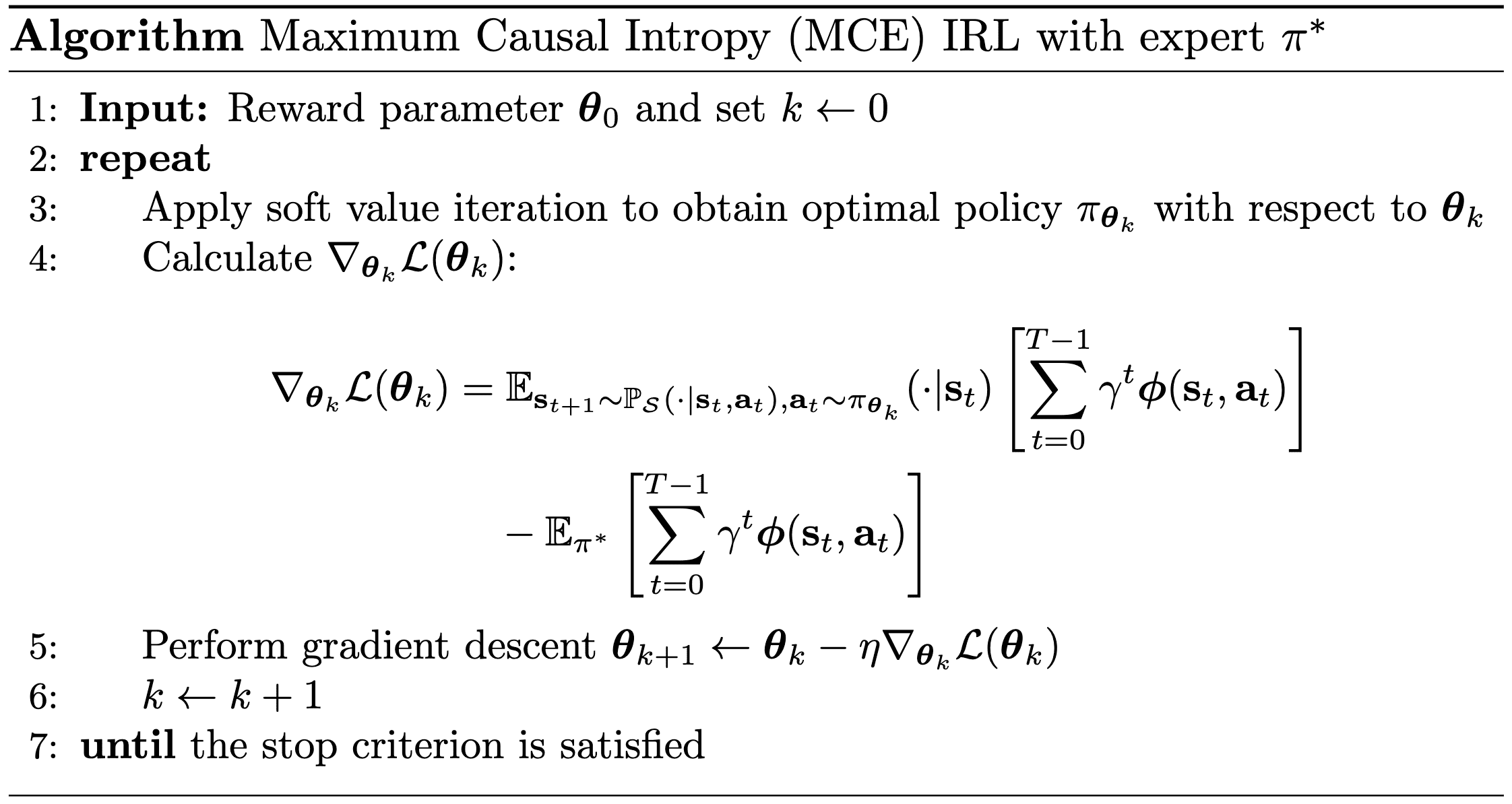
And similar to the original Max-Ent algorithm, we can also interpret this method as maximum likelihood estimation of reward parameters $\boldsymbol{\theta}$ subject to the distribution over trajectories induced by the policy $\pi_\boldsymbol{\theta}$. For mathematical details, please refer to Section 3.2 of Gleave et al. 2022.
References
[1] CS 285 at UC Berkeley, “Deep Reinforcement Learning”
[2] Stanford CS237b, “Principles of Robot Autonomy”
[3] Wikipedia, “Apprenticeship Learning”
[4] Adams et al. “A survey of inverse reinforcement learning”, Artificial Intelligence Review, Volume 55, Issue 6 Pages 4307 - 4346
[5] Arora et al. “A Survey of Inverse Reinforcement Learning: Challenges, Methods and Progress”, arXiv:1806.06877
[6] Zhifei et al. “A survey of inverse reinforcement learning techniques” 2011
[7] Andrew Ng and Stuart Russell, “Algorithms for inverse reinforcement learning”, ICML 2000
[8] Pieter Abbeel and Andrew Ng, “Apprenticeship Learning via Inverse Reinforcement Learning”, ICML 2004
[9] Ratliff et al. “Maximum Margin Planning”, ICML 2006
[10] Ramachandran et al. “Bayesian Inverse Reinforcement Learning”, IJCAI 2007
[11] Chan et al. “Scalable Bayesian Inverse Reinforcement Learning”, ICLR 2021
[12] Ziebart et al. “Maximum Entropy Inverse Reinforcement Learning”, AAAI 2008
[13] Wikipedia, “Maximum entropy probability distribution”
[14] Wainwright, Martin J., and Michael I. Jordan. “Graphical models, exponential families, and variational inference.” Foundations and Trends® in Machine Learning 1.1–2 (2008): 1-305.
[15] Boularias et al. “Relative Entropy Inverse Reinforcement Learning”, PMLR 2011
[16] Ziebart et al. “Modeling Interaction via the Principle of Maximum Causal Entropy”, ICML 2010
[17] Gleave et al. “A Primer on Maximum Causal Entropy Inverse Reinforcement Learning”, arXiv:2203.11409

Leave a comment