[RL] Implicit World Model

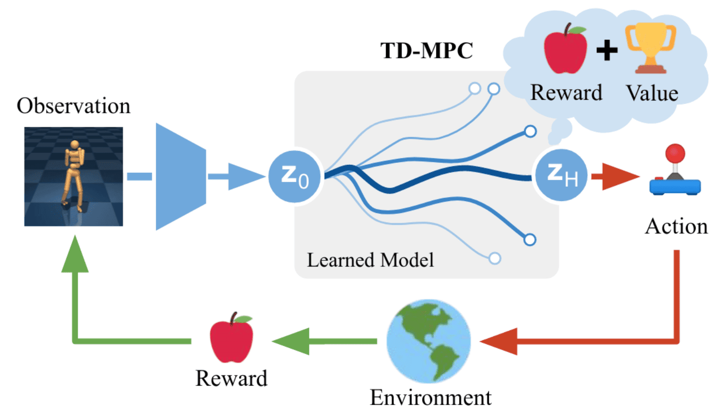
Learning the world model through a reconstruction (decoder) objective is appealing due to its abundant learning signals. However, predicting raw future observations (e.g., images or proprioceptive data) over long time horizons is a challenging problem, and may not lead to efficient control. Instead of explicitly modeling dynamics via reconstruction, TD-MPC and TD-MPC2 focus on learning a maximally useful model that accurately predicts returns conditioned on a sequence of actions. Specifically, they learn an implicit, control-centric world model from environment interactions, using a combination of 3 problems (joint-embedding prediction, reward prediction, and TD-learning) without decoding observations.

$\mathbf{Fig\ 1.}$ TD-MPC framework (Hansen et al. 2022)

Preliminary: Model Predictive Control (MPC)

Model predictive control (MPC) is an optimal control method that plans an optimized sequence of actions in the model. Formally, at time step $t$, an MPC agent seeks an action sequence \(\mathbf{a}_{t:t+\tau}\) by optimizing:

\[\begin{aligned} \max_{\mathbf{a}_{t:t+\tau}} \mathbb{E}_{\mathbf{s}_{t^\prime + 1} \sim \mathcal{T} (\cdot \vert \mathbf{s}_{t^\prime}, \mathbf{a}_{t^\prime})} \left[ \sum_{t^\prime = t}^{t + \tau} r (\mathbf{s}_{t^\prime}, \mathbf{a}_{t^\prime}) \right] \end{aligned}\]

where $\tau$ denotes the planning horizon. The agent then sekects the first action \(\mathbf{a}_t\) from the optimized sequence and applies it to the environment. By executing these action sequences within the model, the current state \(\mathbf{s}_t\) transitions to \(\mathbf{s}_{t+\tau}\) according to the transition distribution $\mathcal{T}$. The returns accumulated during this transition process are used to assess the chosen action sequences.

In general, there are several options for planning the action sequence:

• Monte Carlo sampling of \(\mathbf{a}_{t:t+\tau}\) from the action space uniformly and randomly;
  • e.g., MB-MF
• Cross Entropy Method (CEM), which iteratively refines the distribution of action sequences towards high-reward regions;
  • e.g., PlaNet
• and others.

TD-MPC: Temporal Difference Learning for MPC

Model-based methods can generally be categorized into two approaches, each leveraging distinct advantages of model-based learning:

• Planning
  • (+) offer benefits over a learned policy
  • (-) possible to become prohibitively expensive when applied to long horizons
  • e.g., PlaNet
• World Model
  • (+) enhance the sample efficiency of model-free methods
  • (-) model biases likely to propagate to the policy as well
  • e.g., Dreamer

Consequently, model-based methods have historically found it challenging to outperform simpler, model-free methods in continuous control tasks. Temporal Difference Learning for Model Predictive Control (TD-MPC) is a framework that augment model-based planning with the strengths of model-free learning. It leverages a Task-Oriented Latent Dynamics (TOLD) model and terminal value function, which are learned jointly by TD learning.

Task-Oriented Latent Dynamics (TOLD)

Instead of modeling the environment directly, TOLD model is an implicit world model that learns to only model elements of the environment that are predictive of reward. During training, the agent incrementally improves the TOLD model using data gathered from past environment interactions, while also collecting new data by performing online planning $\Pi_\theta$ of action sequences. (The planner $\Pi_\theta$ will be specified in the next section.)

$\mathbf{Fig\ 2.}$ TOLD model (Hansen et al. 2023)

It consists of the following 5 learned components:

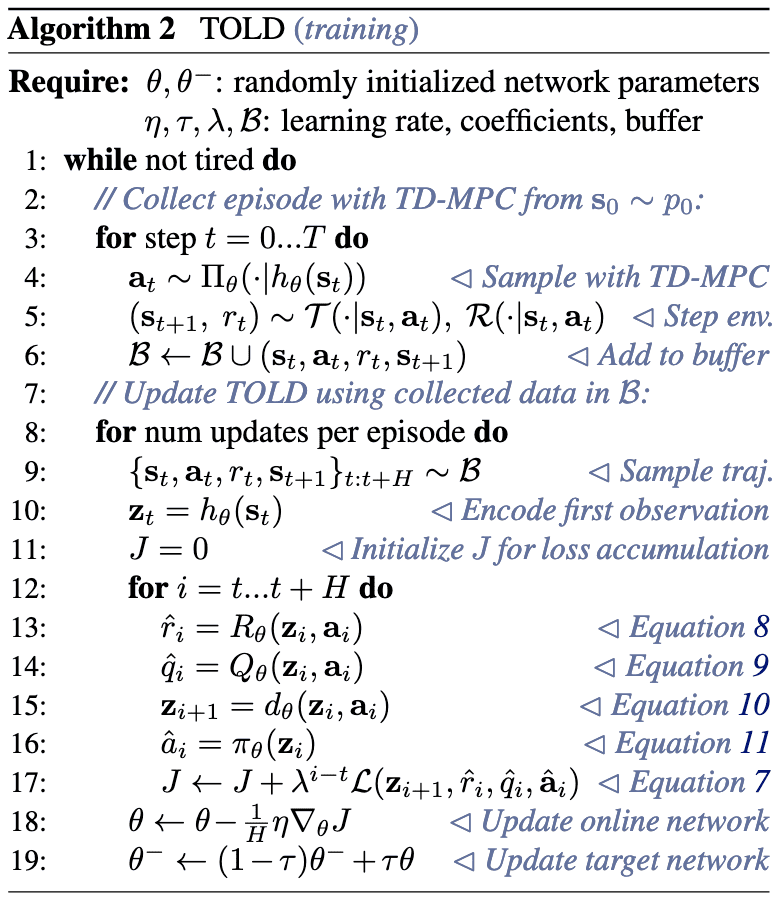
\[\begin{aligned} & \texttt{Representation: } & \mathbf{z}_t = h_\theta (\mathbf{s}_t) \\ & \texttt{Latent Dynamics: } & \mathbf{z}_{t+1} = d_\theta (\mathbf{z}_t, \mathbf{a}_t) \\ & \texttt{Reward: } & \hat{r}_t = R_\theta (\mathbf{z}_t, \mathbf{a}_t) \\ & \texttt{Value: } & \hat{q}_t = Q_\theta (\mathbf{z}_t, \mathbf{a}_t) \\ & \texttt{Policy Prior: } & \hat{\mathbf{a}}_t \sim \pi_\theta (\mathbf{z}_t) \\ \end{aligned}\]

t is worth noting that the authors discovered it is sufficient to implement all components of TOLD as purely deterministic MLPs, i.e., without RNN gating mechanisms or probabilistic models. During training, TD-MPC minimizes a temporally weighted objective:

\[\mathcal{J}(\theta; \Gamma) = \sum_{t^\prime = t}^{t + H} \lambda^{t^\prime - t} \mathcal{L}(\theta; \Gamma_{t^\prime})\]

where \(\Gamma = (\mathbf{s}_t, \mathbf{a}_t, r_t, \mathbf{s}_{t+1})_{t:t+H} \sim \mathcal{B}\) is a sampled trajectory from a replay buffer $\mathcal{B}$ and the single-step loss:

\[\begin{aligned} & \mathcal{L}\left(\theta ; \Gamma_{t^\prime}\right)=c_1 \underbrace{\left\Vert R_\theta\left(\mathbf{z}_{t^\prime}, \mathbf{a}_{t^\prime}\right)-r_{t^\prime}\right\Vert_2^2}_{\text {reward }} \\ & +c_2 \underbrace{\left\Vert Q_\theta\left(\mathbf{z}_{t^\prime}, \mathbf{a}_{t^\prime}\right)-\left(r_{t^\prime}+\gamma Q_{\theta^{-}}\left(\mathbf{z}_{t^\prime+1}, \pi_\theta\left(\mathbf{z}_{t^\prime+1}\right)\right)\right)\right\Vert_2^2}_{\text {value }} \\ & +c_3 \underbrace{\left\Vert d_\theta\left(\mathbf{z}_{t^\prime}, \mathbf{a}_{t^\prime}\right)-h_{\theta^{-}}\left(\mathbf{s}_{t^\prime+1}\right)\right\Vert_2^2}_{\text {latent state consistency }} \end{aligned}\]

that aims to jointly optimize for reward prediction, value prediction, and a latent state consistency loss that regularizes the learned representation. Note that subsequent observations are encoded using EMA target net $h_{\theta^−}$.

1. Value Learning with TD-targets
   Since the TD-objective of TOLD requires the expensive max operation for $\max_{\mathbf{a}_t} Q_{\theta^-} (\mathbf{z}_t, \mathbf{a}_t)$, it instead learns a policy $\pi_\theta$ to take action maximizes the Q-function: $$ \mathcal{J}_\pi (\theta; \Gamma) = -\sum_{t^\prime = t}^{t+H} \lambda^{t^\prime - t} Q_\theta \left(\mathbf{z}_t, \pi_\theta \left(\texttt{sg}(\mathbf{z}_{t^\prime}) \right) \right) $$ Here, $\pi_\theta$ is implemented as a deterministic policy with Gaussian noise applied to actions as in DDPG: $$ \mathbf{a}_t = \texttt{clip} (\pi_\theta (\mathbf{s}_t) + \varepsilon, \mathbf{a}_\texttt{low}, \mathbf{a}_\texttt{high}) \text{ where } \varepsilon \sim \mathcal{N}(\mathbf{0}, \mathbf{I}) $$
2. Latent state consistency
   Learning to predict raw future observations is an exceedingly challenging and inefficient task, as it forces the network to model all aspects of the environment, including task-irrelevant quantities and details such as shading. To address this inefficiency, TOLD utilized latent state consistency loss: $$ \left\Vert d_\theta\left(\mathbf{z}_{t^\prime}, \mathbf{a}_{t^\prime}\right)-h_{\theta^{-}}\left(\mathbf{s}_{t^\prime+1}\right)\right\Vert_2^2 $$ to force the consistency between a future latent space prediction $\mathbf{z}_{t+1} = d_\theta (\mathbf{z}_t, \mathbf{a}_t)$ and the latent of the corresponding observation $h_{\theta^{-}} (\mathbf{s}_{t+1})$.

$\mathbf{Fig\ 3.}$ The pseudocode of training TOLD model (Hansen et al. 2022)

MPC with TOLD model

Throughout inference, the agent then leverages the learned TOLD model for trajectory optimization, estimating short-term rewards using model rollouts and long-term returns using the terminal value function.

Planning with CEM

The authors adapt Cross Entropy Method (CEM) for planning action sequences. More precisely, with initial parameters for each action over a horizon of length $H$ \((\mu^0, \sigma^0)_{t:t+H}\) where \(\mu^0, \sigma^0 \in \mathbb{R}^{\vert \mathcal{A} \vert}\), firstly sample independent $N$ trajectories \(\{ \Gamma_i \}_{i=1}^N\) generated by the learned model $d_\theta$, and estimate the total return $\phi_\Gamma$:

\[\phi_\Gamma = \mathbb{E}_{\mathbf{z}_{t+1} \sim d_\theta (\mathbf{z}_t, \mathbf{a}_t), \mathbf{a}_t \sim \mathcal{N} (\mu_t^{j - 1}, ( \sigma_t^{j-1})^2 \mathbf{I})} \left[ \sum_{h=0}^{H-1} \gamma^h R_\theta (\mathbf{z}_{t + h}, \mathbf{a}_{t + h}) + \gamma^H Q_\theta (\mathbf{z}_{t+H}, \mathbf{a}_{t+H}) \right]\]

at iteration $j - 1$. Then, obtain new parameter $(\mu^j, \sigma^j)_{t:t+H}$ at iteration $j$ by empirical estimates from trajectories \(\{ \Gamma_i^\star \}_{i=1}^k\) with top-$k$ returns \(\phi_\Gamma^\star\):

\[\mu_{t^\prime}^j = \frac{\sum_{i=1}^k w_i \mathbf{a}_{i, t^\prime}^\star}{\sum_{i=1}^k w_i}, \quad \sigma_{t^\prime}^j = \sqrt{\frac{\sum_{i=1}^k w_i (\mathbf{a}_{i, t^\prime}^\star - \mu_{t^\prime}^j)^2}{\sum_{i=1}^k w_i}}\]

where $w_i = \exp (\tau \cdot \phi_{\Gamma_{i}^\star})$ with sharpness temperature parameter $\tau$ and \(\Gamma_i^\star = (\mathbf{z}_{i, t}^\star, \mathbf{a}_{i, t}^\star, \cdots \mathbf{z}_{i, t+H}^\star, \mathbf{a}_{i, t+H}^\star)\).

The planning horizon is linearly increased from $1$ to $H$ in the early stages of training, as the model is initially inaccurate and planning would therefore be dominated by model bias.

Exploration

The authors observed that the rate at which $\sigma$ decays varies wildly between tasks, leading to (potentially poor) local optima for small $\sigma$. To promote consistent exploration across tasks, they constrained $\sigma^j$ such that:

\[\sigma_{t^\prime}^j = \sqrt{\frac{\sum_{i=1}^k w_i (\mathbf{a}_{i, t^\prime}^\star - \mu_{t^\prime}^j)^2}{\sum_{i=1}^k w_i}} = \max \left( \sqrt{\frac{\sum_{i=1}^k w_i (\mathbf{a}_{i, t^\prime}^\star - \mu_{t^\prime}^j)^2}{\sum_{i=1}^k w_i}}, \epsilon \right)\]

where $\epsilon \in \mathbb{R}_{>0}$ is a linearly decayed constant.

$\mathbf{Fig\ 4.}$ The pseudocode of TD-MPC inference (Hansen et al. 2022)

Experimental Results

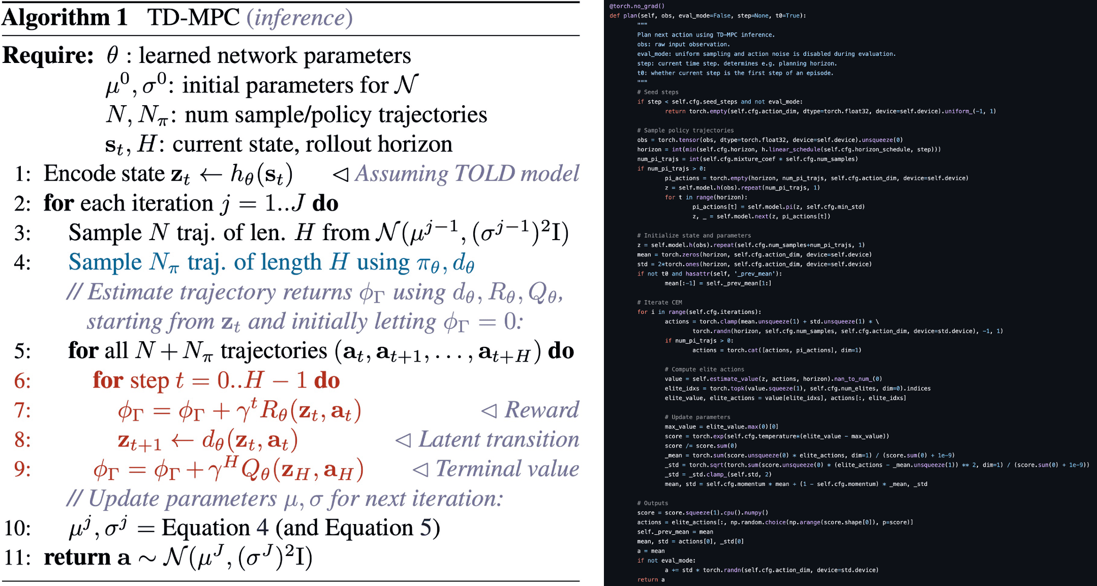
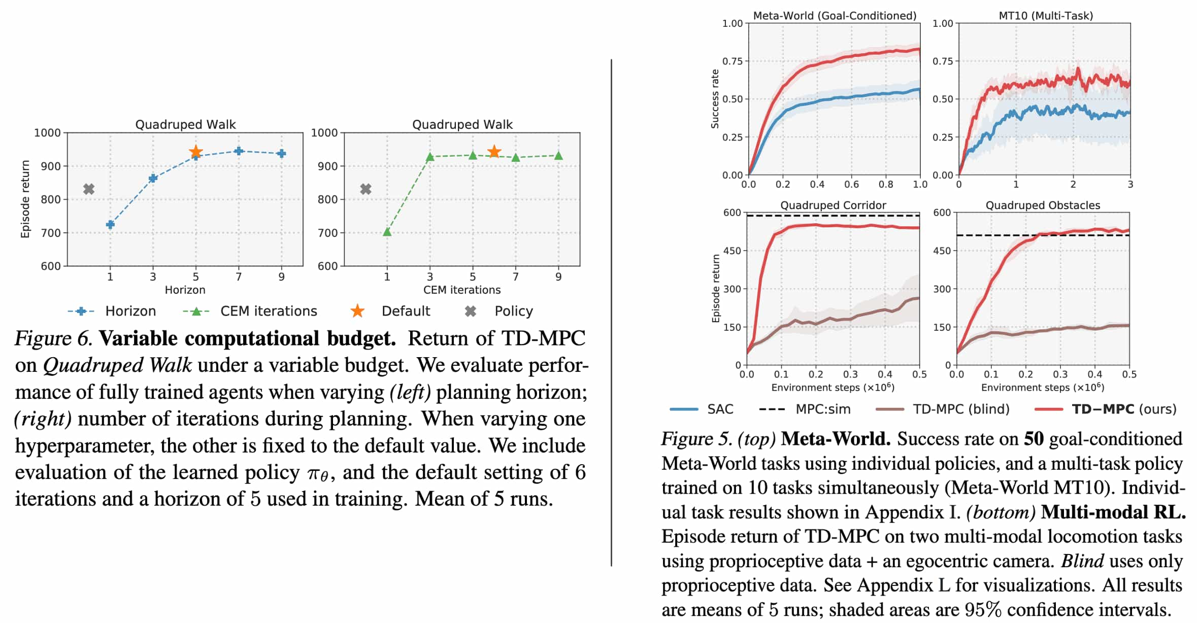
As a result, TD-MPC, achieves superior sample efficiency and asymptotic performance over prior work on both state and image-based continuous control tasks from DMControl and Meta-World.

$\mathbf{Fig\ 5.}$ DMControl Performances (Hansen et al. 2022)

$\mathbf{Fig\ 6.}$ Meta-World Performances (Hansen et al. 2022)

TD-MPC2: Scalable, Robust World Models for Continuous Control

TD-MPC2 represents a series of improvements to the TD-MPC algorithm. Its single hyperparameter agent has demonstrated scalable and robust performance across 80 tasks spanning various task domains, embodiments, and action spaces. In summary, the main differences between TD-MPC and TD-MPC2 are as following:

• Architectural Design with $\texttt{SimNorm}$
• Soft Actor-Critic (SAC) Policy Prior
• Model Objective with discrete regression and an ensemble of TD-target
• Multi-task TOLD model

$\mathbf{Fig\ 7.}$ TD-MPC2 compares favorably to existing model-free and model-based RL methods across 104 continuous control tasks spanning multiple domains, with a single set of hyperparameters (Hansen et al. 2024)

Architectural Design

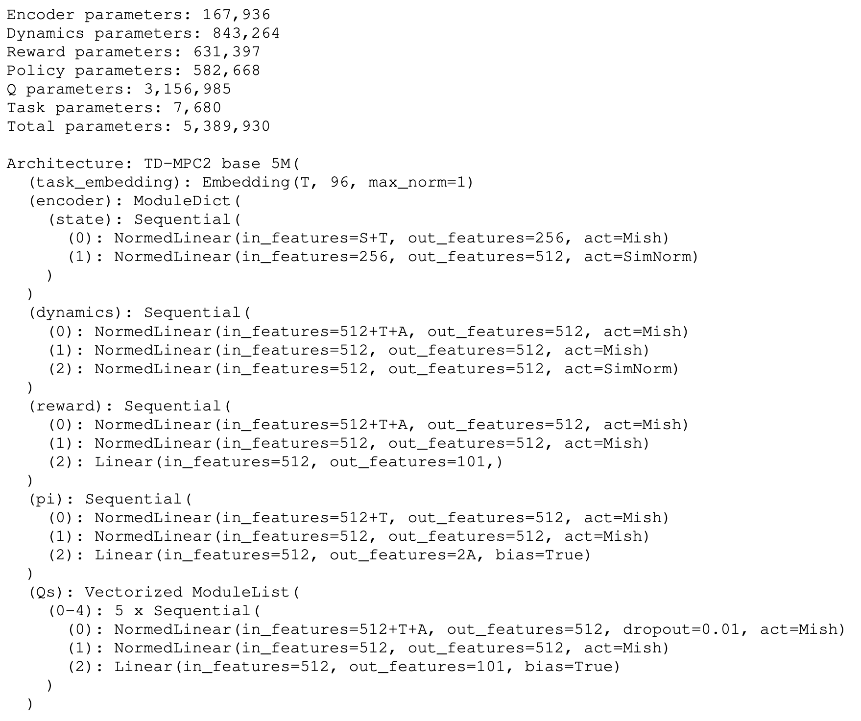
All components of TD-MPC2 are implemented as MLPs with intermediate linear layers followed by LayerNorm and Mish activations:

\[\begin{aligned} \texttt{LayerNorm} (x) & = \frac{x - \mathbb{E}[x]}{\sqrt{\mathrm{Var}[x] + \epsilon}} \cdot \gamma + \beta \\ \texttt{Mish}(x) & = x \cdot \tanh (\texttt{softplus} (x)) \quad \text{ where } \quad \texttt{softplus} (x) = \ln (1 + \exp(x)) \end{aligned}\]

$\mathbf{Fig\ 8.}$ Architectural details of TD-MPC2 (Hansen et al. 2024)

Simplicial Normalization (SimNorm)

To mitigate exploding gradients, the authors proposed the normalization of the latent representation $\mathbf{z}$ called Simplicial Normalization (SimNorm), which projects $\mathbf{z} \in \mathbb{R}^{V \times L}$ into $L$ fixed-dimensional simplices using a softmax operation:

\[\texttt{SimNorm} (\mathbf{z}) = \texttt{concat}(\mathbf{g}_1, \cdots, \mathbf{g}_L)\]

where $V$ is the dimensionality of each simplex $\mathbf{g}$ constructed from $L$ partitions of $\mathbf{z}$ and:

\[\mathbf{g}_i = \texttt{softmax} (\mathbf{z}_{i: i + V}) = \frac{e^{\mathbf{z}_{i:i+V} / \tau}}{\sum_{j=1}^V e^{\mathbf{z}_{i:i+V, j} / \tau}}\]

This normalization can be PyTorch-like implemented as follows:

def simnorm(self, z, V=8):
  shape = z.shape
  z = z.view(*shape[:-1], -1, V)
  z = softmax(z, dim=-1)
  return z.view(*shape)

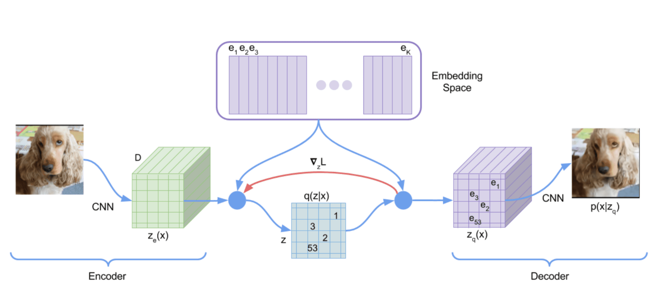
A significant advantage of embedding $\mathbf{z}$ as simplices is that it naturally biases the representation towards sparsity without enforcing hard constraints. Conceptually, it can be regarded as a “soft” version of the vector-of-categoricals method in VQ-VAE, analogous to how $\texttt{softmax}$ serves as a relaxation of the $\arg \max$ operator. While VQ-VAE encodes latent variables using a set of discrete codes ($L$ vector partitions each consisting of a one-hot encoding), SimNorm divides the latent state into $L$ vector partitions of continuous indices that each sum to $1$ with $\texttt{softmax}$.

Note that a temperature parameter $\tau \in [0, \infty]$ regulates the sparsity. For instance, $\tau \to \infty$ would concentrate all probability mass on individual categories, resulting in the discrete codes (one-hot encodings) in VQ-VAE. Conversely, $\tau = 0$ would produce trivial representations with uniform probability mass, prohibiting the propagation of information. Thus, SimNorm encourages sparsity in the representation without resorting to discrete codes or other rigid constraints.

$\mathbf{Fig\ 9.}$ VQ-VAE framework (source: Van Den Oord et al. NeurIPS 2017)

Soft Actor-Critic (SAC) Policy Prior

Similar to TD-MPC, the TOLD model of TD-MPC2 also consists of 5 components:

\[\begin{array}{llll} \text { Encoder } & \mathbf{z}=h(\mathbf{s}, \mathbf{e}) & \triangleright \text { Maps observations to their latent representations } \\ \text { Latent dynamics } & \mathbf{z}^{\prime}=d(\mathbf{z}, \mathbf{a}, \mathbf{e}) & \triangleright \text { Models (latent) forward dynamics } \\ \text { Reward } & \hat{r}=R(\mathbf{z}, \mathbf{a}, \mathbf{e}) & \triangleright \text { Predicts reward } r \text { of a transition } \\ \text { Terminal value } & \hat{q}=Q(\mathbf{z}, \mathbf{a}, \mathbf{e}) & \triangleright \text { Predicts discounted sum of rewards (return) } \\ \text { Policy prior } & \hat{\mathbf{a}}=p(\mathbf{z}, \mathbf{e}) & \triangleright \text { Predicts action } \mathbf{a}^* \text { that maximizes } Q \end{array}\]

where $\mathbf{e}$ is a learnable task embedding for use in multitask world models. Recall that the policy prior $p$ serves to guide the sample-based trajectory optimizer (planner) by saving the sample transitions in the buffer $\mathcal{B}$ and to reduce the computational cost of the $\max$ operator in TD-learning.

$\mathbf{Fig\ 10.}$ The TD-MPC2 architecture (Hansen et al. 2024)

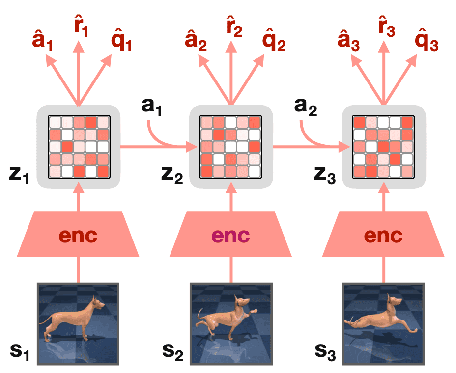
While the policy prior of TD-MPC is trained as a DDPG policy, TD-MPC2 trains $p$ with maximum entropy RL as in soft actor-critic (SAC)

\[\mathcal{L}_p (\theta) = \mathbb{E}_{\tau \sim \mathcal{B}} \left[ \sum_{t=0}^H \lambda^t \left(\alpha \cdot Q (\mathbf{z}_t, p (\mathbf{z}_t)) - \beta \cdot \mathbb{H}[p(\cdot \vert \mathbf{z}_t)] \right) \right] \\ \text{where } \mathbf{z}_{t+1} = d (\mathbf{z}_t, \mathbf{a}_t), \mathbf{z}_0 = h (\mathbf{s}_0)\]

where $\mathbb{H}$ is the entropy of $p$ which can be computed in closed form and

\[\mathbf{a}_t = p (\epsilon_t; \mathbf{s}_t) = \tanh (\mu_\theta (\mathbf{s}_t) + \sigma_\theta (\mathbf{s}_t) \odot \epsilon_t) \text{ where } \epsilon_t \sim \mathcal{N} (\mathbf{0}, \mathbf{I})\]

Although the authors noted that a DDPG policy prior with finely tuned noise scheduling can perform comparably to this SAC policy prior, they chose to adopt maximum entropy RL, as it allows for easier application with task-agnostic hyperparameters (e.g., automatically adjusting $\alpha, \beta$ using moving statistics).

Model Objective

To improve the robustness to variation in tasks, TD-MPC2 modifies several components of TOLD objective. First, the continuous regression of reward and value learning using $L_2$ loss in TD-MPC are replaced by discrete regression (multi-class classification) in a log-transformed space, optimized by cross-entropy loss:

\[\mathcal{L}(\theta) = \mathbb{E}_{(\mathbf{s}, \mathbf{a}, r, \mathbf{s}^{\prime})_{0: H} \sim \mathcal{B}} \left[ \sum_{t=0}^H \lambda^t \times \left(\underbrace{\left\Vert \mathbf{z}_t^{\prime}-\texttt{sg}\left(h(\mathbf{s}_t^{\prime})\right)\right\Vert_2^2}_{\text {Joint-embedding prediction }} + \underbrace{\mathrm{CE}\left(\hat{r}_t, r_t\right)}_{\text {Reward prediction }}+\underbrace{\mathrm{CE}\left(\hat{q}_t, q_t\right)}_{\text {Value prediction }} \right) \right]\]

where

\[q_t = r_t + \gamma \bar{Q} (\mathbf{z}_t^\prime, p (\mathbf{z}_t^\prime))\]

This ensures the magnitude of the two loss terms remains independent of the magnitude of the task rewards, which helps simplify the design of robust reward normalization schemes. TD-MPC2 retains the continuous regression term for joint-embedding prediction, as the latent representation is already normalized by $\texttt{SimNorm}$, and discrete regression would be computationally expensive for high-dimensional spaces.

Ensemble of TD-target

Moreover, to reduce bias in TD-targets generated by $\bar{Q}$, it learns an ensemble of Q-functions (e.g., $5$ Q-functions) using the model objective and maintain $\bar{Q}$ as an EMA of each Q-function. Targets are then computed as the minimum of two randomly sub-sampled $\bar{Q}$-functions, similar to clipped double Q-learning of TD3.

Training Multi-task Model

To succeed in a multitask setting, an agent must learn a common representation that leverages task similarities while maintaining the capacity to distinguish between tasks during test time. Additionally, the agent should be capable of performing tasks across a range of observation and action spaces, without relying on any domain knowledge. To achieve this, TD-MPC2 incorporates the following additional techniques:

1. Learnable task embeddings
   TD-MPC2 conditions all of its five components with a learnable, fixed-dimensional task embedding $\mathbf{e}$, which is jointly trained together with other components of the model from data. To improve training stability, the $L_2$ norm of $\mathbf{e}$ is constrained to be $\leq 1$.
2. Action masking
   TD-MPC2 zero-pads all model inputs and outputs to their largest respective dimensions, and mask out invalid action dimensions in predictions made by the policy prior $p$ during both training and inference. This ensures that prediction errors in invalid dimensions do not influence TD-target estimation, and prevents $p$ from falsely inflating its entropy for tasks with small action spaces.

Experimental Results

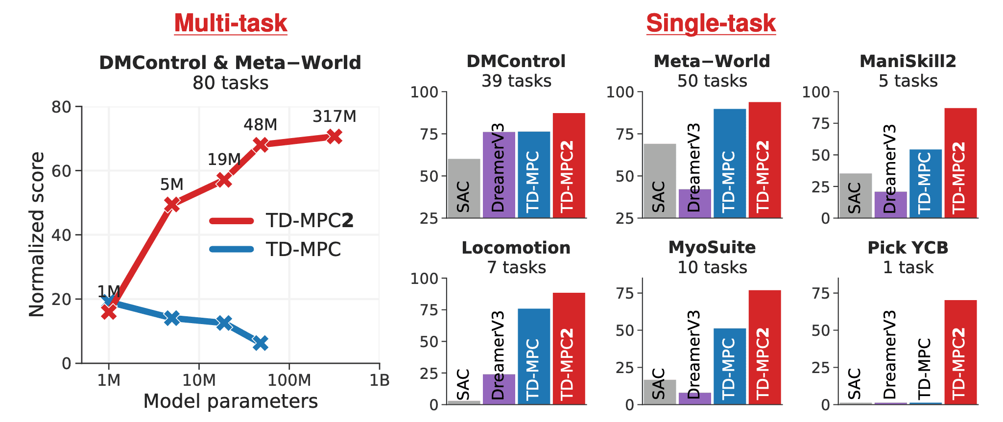
On 104 diverse tasks in an online RL, TD-MPC2 outperforms prior methods across all task domains.

$\mathbf{Fig\ 11.}$ Single-task RL (Hansen et al. 2024)

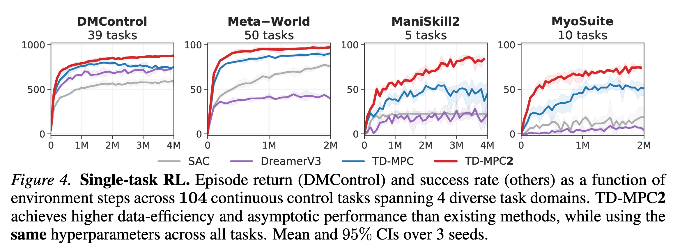
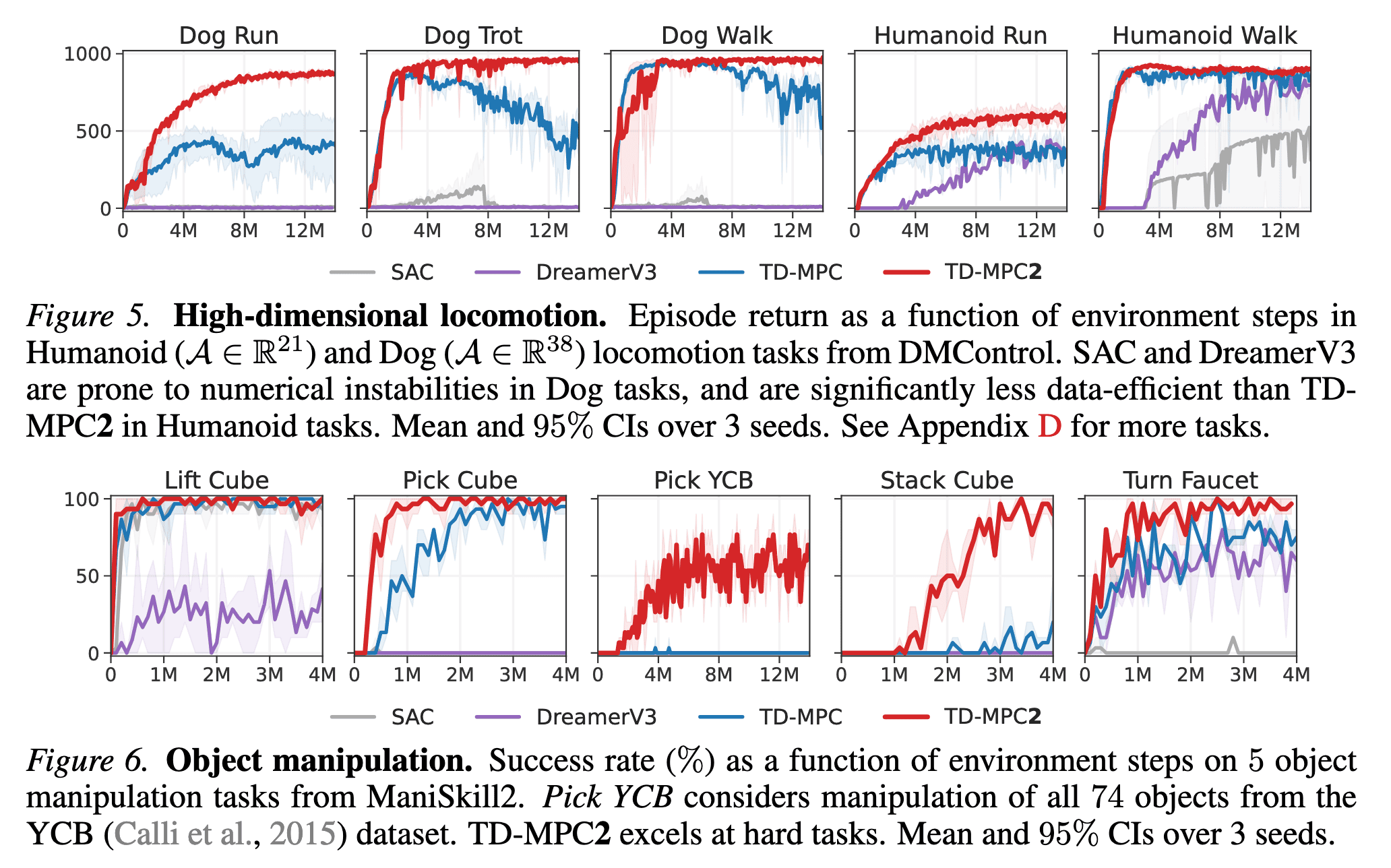
In some of the most challenging tasks (high-dimensional locomotion and multi-object manipulation), TD-MPC2 significantly outperforms baselines on these tasks, despite using the same hyperparameters across all tasks.

$\mathbf{Fig\ 12.}$ Comparisons on difficult tasks (Hansen et al. 2024)

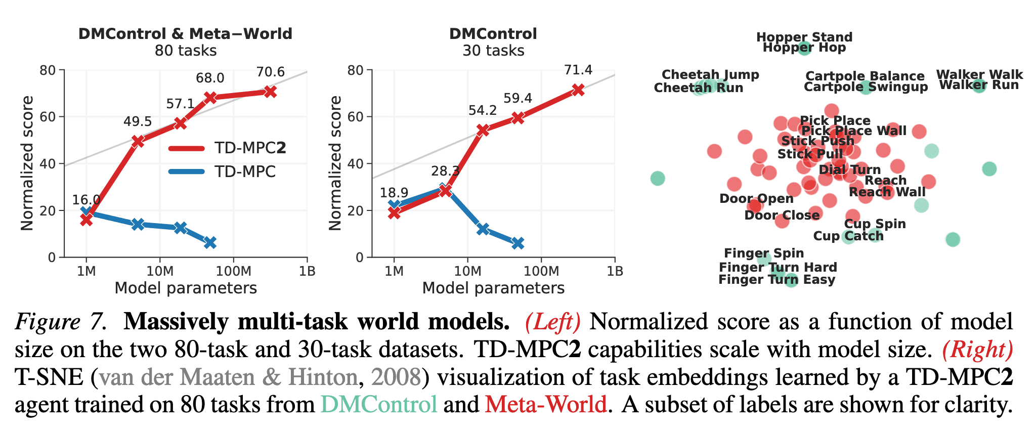
To demonstrate that TD-MPC2 facilitates the scaling of world models, the authors evaluate the performance of five multi-task models ranging from $1\textrm{M}$ to $317\textrm{M}$ parameters across a collection of $80$ diverse tasks that span multiple task domains and vary significantly in objective, embodiment, and action space. To summarize agent performance with a single metric, they calculate a normalized score that averages all individual task success rates (Meta-World) and episode returns, which are normalized to the $[0, 100]$ range (DMControl).

Consequently, the authors observe that agent capabilities consistently improve with model size across both task sets. Furthermore, t-SNE analysis of task embeddings reveals that the task embeddings are learned in accordance with our intended behavior. It is revealed that task embeddings are tightly coupled with control, since tasks that are semantically similar are close in the learned task embedding space.

$\mathbf{Fig\ 13.}$ Massively multi-task world models (Hansen et al. 2024)

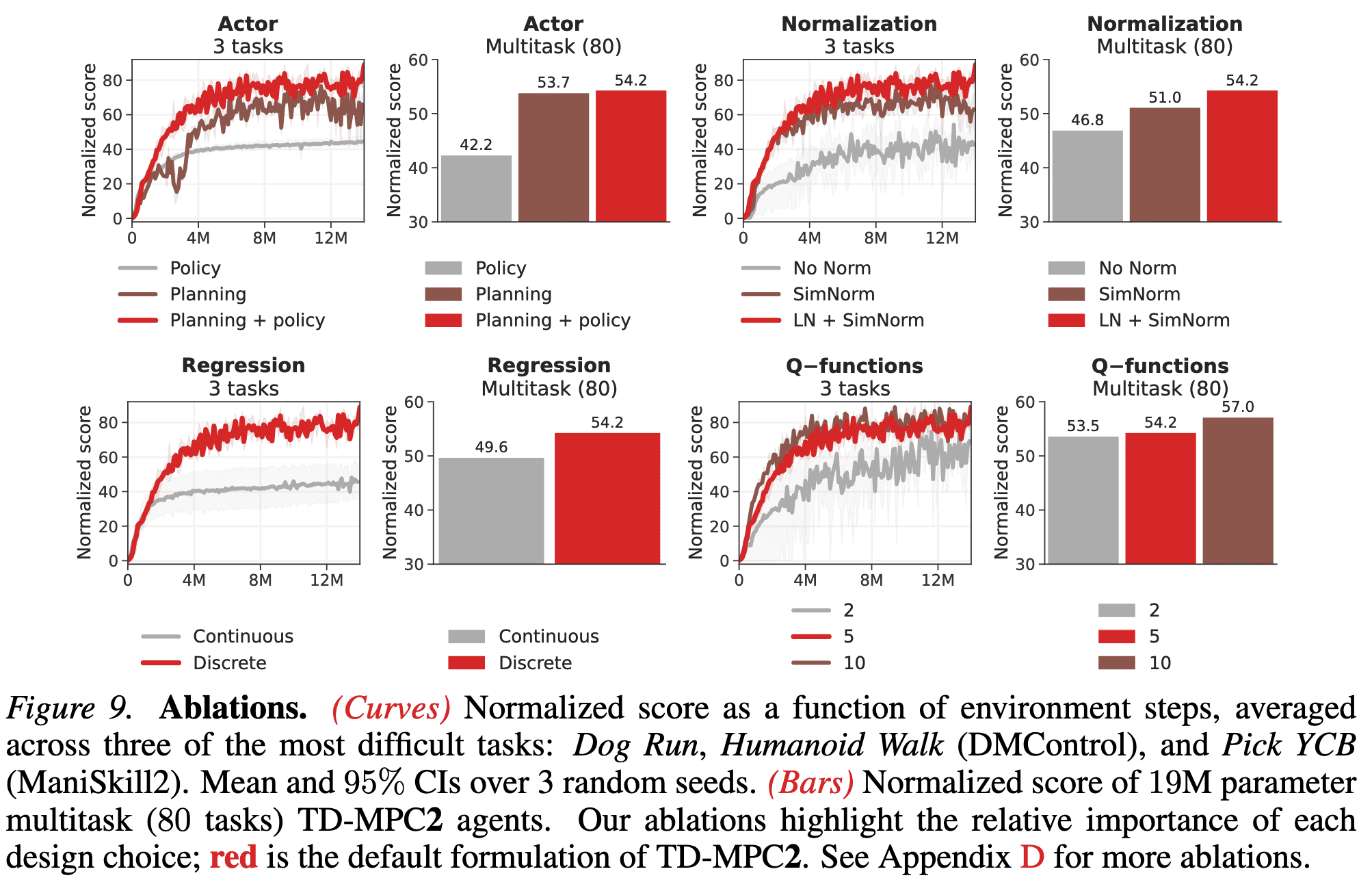
The following figure shows the ablation of most of our design choices for TD-MPC2, including choice of actor, various normalization techniques, regression objective, and number of Q-functions.

$\mathbf{Fig\ 14.}$ TD-MPC2 Ablations (Hansen et al. 2024)

References

[1] Hansen et al. “Temporal Difference Learning for Model Predictive Control”, ICML 2022
[2] Hansen et al. “TD-MPC2: Scalable, Robust World Models for Continuous Control”, ICLR 2024