[RL] Self-Predictive RL

In deep reinforcement learning, a multitude of representation learning methods have been proposed, ranging from state representations for MDPs to history representations for POMDPs. However, these approaches often differ in their learning objectives and training techniques, making it difficult for users to choose the most appropriate method for their specific problems.

Recently, Ni et al., ICLR 2024 provided a unified perspective on various representations proposed in earlier works, demonstrating that many seemingly distinct methods and frameworks are, in fact, all connected through a self-predictive learning–where the encoder is capable of predicting its subsequent latent state. This post explores this self-predictive aspects of prior works, and also introduces one of the most popular instances called SPR, proposed by Schwarzer et al., 2021, for a deeper understanding.

$\mathbf{Fig\ 1.}$ SPR framework (Schwarzer et al. 2021)

Abstraction Theory for MDP

Previous works on representation learning in RL define different encoders based on the observability of MDP. In a POMDP, the agents derive advantages from the observed history \(\mathbf{h}_t := (\mathbf{h}_{t-1}, \mathbf{a}_{t-1}, \mathbf{o}_t) \in \mathcal{H}_t\) with an encoder $\phi: \mathcal{H}_t \to \mathcal{Z}$ that generates a history representation \(\mathbf{z} = \phi(\mathbf{h}) \in \mathcal{Z}\). Likewise, in a fully observable MDP, $\mathbf{h}$ is replaced with $\mathbf{s}$, leading to a state encoder $\phi: \mathcal{S} \to \mathcal{Z}$ and a state representation $\mathbf{z} = \phi(\mathbf{s}) \in \mathcal{Z}$.

Additionally, these encoders are often shared and jointly updated by downstream components (e.g., policy, value, world model) of an RL system.

Abstraction Theory

As Li et al. 2006 define, abstraction can be understood as the process of mapping a ground representation–the original, detailed description of a problem–to a more abstract, compact representation that is easier to work with. And the abstraction theory defines what kind of abstraction we seek to achieve.

X-abstraction: The encoder provides an X-abstraction if it preserves all necessary information required for X.

Representation learning is intimately connected to abstraction theory, as it seeks to encode large inputs into more compact embeddings while retaining the essential information needed for the tasks at hand. Then, what kind of information should be preserved in RL?

1. $Q^*$-irrelevance abstraction $\phi_{Q^*}$
   We want an encoder $\phi_{Q^*}$ that preserves necessary information for predicting the true return $Q^*$: $$ \phi_{Q^*} (\mathbf{h}_t) = \phi_{Q^*} (\mathbf{h}_{t^\prime}) \implies \forall \mathbf{a} \in \mathcal{A}: Q^* (\mathbf{h}_t, \mathbf{a}) = Q^* (\mathbf{h}_{t^\prime}, \mathbf{a}) $$ Usually, this abstraction can be achieved by default in end-to-end model-free algorithms (e.g., DQN, SAC) through a value function $Q(\phi (\mathbf{h}), \mathbf{a})$.
2. Self-predictive (Model-irrelevance) abstraction $\phi_L$
   We want an encoder $\phi_L$ that preserves necessary information for predicting environment dynamics (reward + transition dynamics), i.e. for expected reward prediction (RP) and next latent ($\mathbf{z}$) distribution prediction (ZP). We will label these properties as RP and ZP, respectively. $$ \begin{aligned} & \exists R_\mathbf{z}: \mathcal{Z} \times \mathcal{A} \rightarrow \mathbb{R}, \quad \text { s.t. } \quad \mathbb{E}[r \mid \mathbf{h}, \mathbf{a}] = R_\mathbf{z} (\phi_L(\mathbf{h}), \mathbf{a}), \quad \forall \mathbf{h}, \mathbf{a} & \textrm{(RP)} \\ & \exists P_\mathbf{z}: \mathcal{Z} \times \mathcal{A} \rightarrow \Delta(\mathcal{Z}), \quad \text { s.t. } \quad P (\mathbf{z}^{\prime} \mid \mathbf{h}, \mathbf{a}) = P_\mathbf{z} (\mathbf{z}^{\prime} \mid \phi_L(\mathbf{h}), \mathbf{a} ), \quad \forall \mathbf{h}, \mathbf{a}, \mathbf{z}^{\prime} & \textrm{(ZP)} \\ & \mathbb{E}\left[\mathbf{z}^{\prime} \mid \mathbf{h}, \mathbf{a}\right]=\mathbb{E}\left[\mathbf{z}^{\prime} \mid \phi_L(h), \mathbf{a}\right], \quad \forall \mathbf{h}, \mathbf{a} & \textrm{(EZP)} \end{aligned} $$ The expected next latent state $\mathbf{z}$ prediction (EZP) condition is a weak version of ZP.
3. Observation-predictive (belief) abstraction $\phi_O$
   We want an encoder $\phi_O$ that preserves necessary information for predicting environment dynamics and its observations, i.e. for expected reward prediction (RP), next observation ($\mathbf{o}$) prediction (OP) and is a recurrent encoder (Rec). $$ \begin{aligned} & \exists \psi_\mathbf{z}: \mathcal{Z} \times \mathcal{A} \times \mathcal{O} \rightarrow \mathbb{R}, \quad \text { s.t. } \quad \phi(\mathbf{h}^\prime) = \psi_\mathbf{z} (\phi_O (\mathbf{h}), \mathbf{a}, \mathbf{o}^\prime) \quad \forall \mathbf{h}, \mathbf{a}, \mathbf{o}^\prime & \textrm{(Rec)} \\ & \exists P_\mathbf{o}: \mathcal{Z} \times \mathcal{A} \rightarrow \Delta(\mathcal{O}), \quad \text { s.t. } \quad P (\mathbf{o}^{\prime} \mid \mathbf{h}, \mathbf{a}) = P_\mathbf{o} (\mathbf{o}^{\prime} \mid \phi_O(\mathbf{h}), \mathbf{a} ), \quad \forall \mathbf{h}, \mathbf{a}, z^{\prime}, \mathbf{o}^\prime & \textrm{(OP)} \\ & \exists \psi_\mathbf{o}: \mathcal{Z} \rightarrow \mathbb{O}, \quad \text { s.t. } \quad \mathbf{o} = \psi_\mathbf{o} (\phi_O (\mathbf{h})), \quad \forall \mathbf{h} & \textrm{(OR)} \end{aligned} $$ The OP is closely related to observation reconstruction (OR), widely used in practice. Also, the Rec condition is satisfied for encoders parameterized with feedforward or recurrent neural networks, but not Transformers.

Implication Graph of Representations in RL

Ni et al. 2024 demonstrated that these conditions and abstractions can imply one another. And they showed that many of these seemingly distinct methods and frameworks are, in fact, all unified by a self-predictive condition (ZP), where the encoder can predict its subsequent latent state.

$\mathbf{Fig\ 2.}$ Implication graph (Ni et al. 2024)

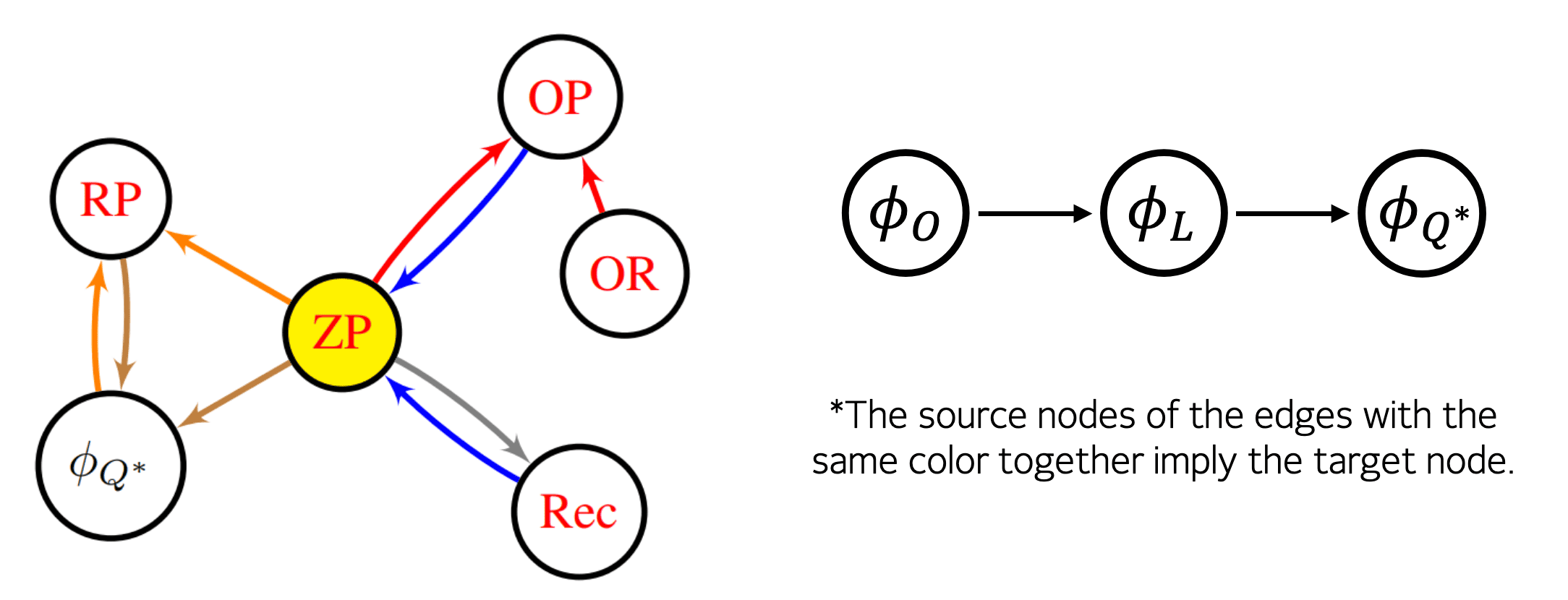
For example, the following theorem, proved by Ni et al. 2024, suggests that if we learn an encoder $\phi_L$ end-to-end in a model-free manner while achieving ZP as an auxiliary task, the ground-truth expected reward can be derived from the latent Q-value and latent transition, which isa crucial element in maximizing the true return.

$\color{red}{\mathbf{Thm.}}$ ZP + $\phi_{Q^*}$ imply RP
If an encoder $\phi$ satisfies ZP, and $Q(\phi (\mathbf{h}), \mathbf{a}) = Q^* (\mathbf{h}, \mathbf{a})$ for all $\mathbf{h}$, $\mathbf{a}$, then we can construct a latent reward function $\mathcal{R}_\mathbf{z} := Q (\mathbf{z}, \mathbf{a}) - \gamma \mathbb{E}_{\mathbf{z}^\prime \sim P_\mathbf{z}(\cdot \mathbf{z}, \mathbf{a})} [\max_{\mathbf{a}^\prime} Q (\mathbf{z}^\prime, \mathbf{a}^\prime)]$, such that $\mathcal{R}_\mathbf{z} (\phi (\mathbf{h}), \mathbf{a}) = \mathbb{E} [r (\mathbf{h}, \mathbf{a})]$.

Self-Predictive RL

While self-predictive representation offers great potential, it presents significant learning challenges compared to grounded model-free and observation-predictive representations. The bootstrapping effect, where $\phi$ appears on both sides of ZP condition (since $\mathbf{z}^\prime$ depends on $\phi(\mathbf{h}^\prime)$), exacerbates this difficulty. Ni et al. 2024 provided some clues for this; the stop-gradient technique, where the encoder’s parameters remain fixed when used as a target, holds promise for learning the desired condition without representational collapse.

Previous works have introduced several auxiliary losses, as summarized in the ZP loss column of the following table. Formally, these works can be categorized into two main approaches: deterministic $\ell_2$ method (with cosine similarity also falling under this category, as $\ell_2$​ distance is equivalent to cosine distance in a normalized vector space) and the probabilistic $f$-divergence method, which includes forward and reverse KL divergences (abbreviated as FKL and RKL).

\[\begin{aligned} \mathcal{L} (\theta, \phi) & := \mathbf{E}_{\mathbf{o}^\prime \sim P (\cdot \vert \mathbf{h}, \mathbf{a})} \left[ \Vert g_\theta (f_\phi (\mathbf{h}), \mathbf{a}) - f_{\bar{\phi}} (\mathbf{h}^\prime) \Vert_2^2 \right] \\ \mathcal{L} (\theta, \phi) & := \mathbf{E}_{\mathbf{z} \sim \mathbb{P}_\phi (\cdot \vert \mathbf{h}), \mathbf{o}^\prime \sim P (\cdot \vert \mathbf{h}, \mathbf{a})} \left[ D_f \left(\mathbb{P}_{\bar{\phi}} (\mathbf{z}^\prime \vert \mathbf{h}^\prime) \Vert \mathbb{P}_\theta (\mathbf{z}^\prime \vert \mathbf{z}, \mathbf{a}) \right) \right] \\ \end{aligned}\]

where $\bar{\phi}$, called ZP target in the paper, is the stop-gradient version of $\phi$:

\[\begin{gathered} \bar{\phi} \leftarrow \tau \bar{\phi} + (1-\tau) \phi \\ \begin{cases} \tau = 0 & \quad \texttt{detached} \\ \tau \in (0,1) & \quad \texttt{EMA} \end{cases} \end{gathered}\]

$\mathbf{Fig\ 3.}$ Which optimal representation will be learned by the value function in prior works? (Hansen et al. 2022)

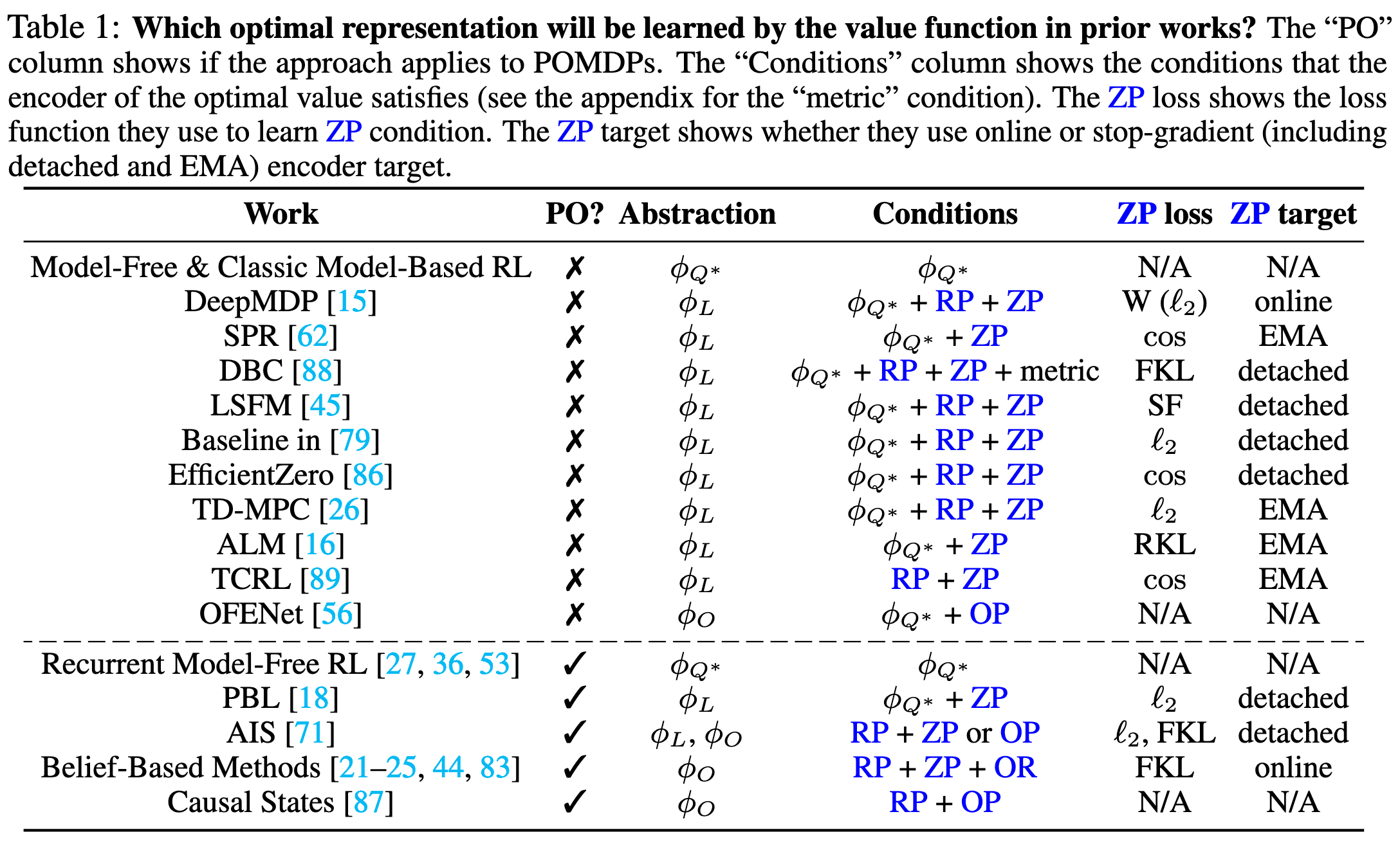
Ni et al. 2024 shows that the widely used stop-gradient (detached or EMA) ZP targets play an important role in optimization that stop-gradient can avoid representational collapse under some linear assumptions, while online ZP targets lack these properties.

$\color{red}{\mathbf{Thm.}}$ Stop-gradient provably avoids representational collapse in linear models
Assume a linear encoder $f_\phi (\mathbf{h}) = \phi^\top \mathbf{h_{-k:}} \in \mathbb{R}^d$ with parameters $\phi \in \mathbb{R}^{k (\vert \mathcal{O} \vert + \vert \mathcal{A} \vert) \times d}$, which always operates on a recent-$k$ truncation of history $\mathbf{h}$, $\mathbf{h}_{-k:}$. Assume a linear deterministic latent transition $g_\theta (\mathbf{z}, \mathbf{a}) := \theta_\mathbf{z}^\top \mathbf{z} + \theta_\mathbf{a}^\top \mathbf{a} \in \mathbb{R}^d$ with parameters $\theta_\mathbf{z} \in \mathbb{R}^{d \times d}$ and $\theta_\mathbf{a} \in \mathbb{R}^{\vert \mathcal{A} \vert \times d}$.
If we train $(\phi, \theta)$ using the stop-gradient $\ell_2$ objective $\mathbb{E}_{\mathbf{h}, \mathbf{a}} [\mathcal{L} (\theta, \phi)]$ and $\theta$ relies on $\phi$ by reaching the stationary point with $\nabla_\theta \mathbb{E}_{\mathbf{h}, \mathbf{a}} [\mathcal{L} (\theta, \phi)] = 0$, then the matrix multiplication $\theta^\top \theta$ will retain its initial value over continuous-time training dynamics.

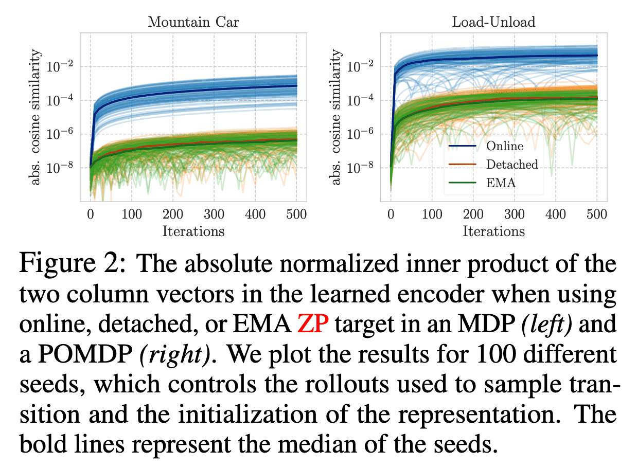
In other words, this theorem implies that the initialized rank of $\phi$ is retained during training by the mathematical fact $\text{rank}(A^\top A) = \text{rank} (A)$. This theorem is also empirically validated in the following figure. The cosine similarity between the columns of the learned $\phi$ is several orders of magnitude smaller when employing the stop-gradient technique (either detached or using EMA) compared to the online case.

$\mathbf{Fig\ 4.}$ The absolute normalized inner product of the two column vectors in the learned linear encoder (Schwarzer et al. 2021)

Self-Predictive Representations (SPR)

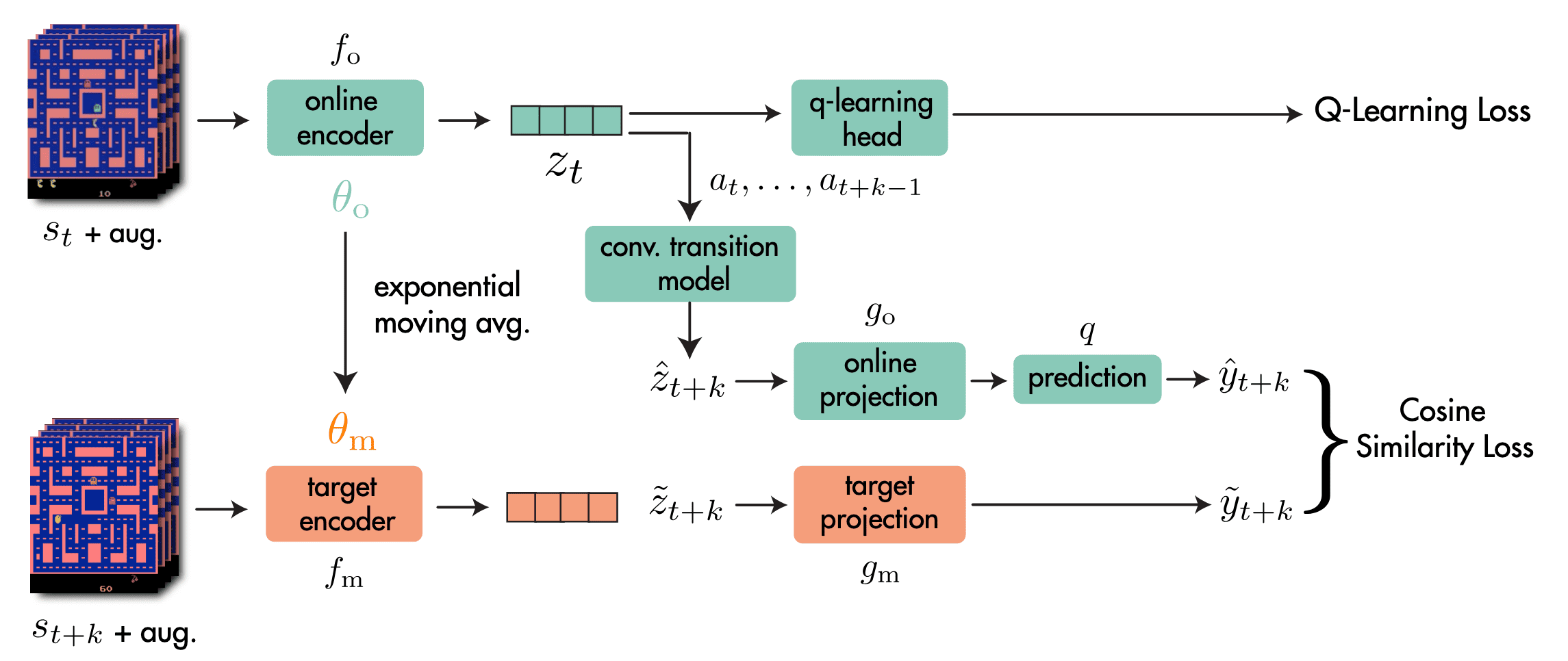
The most prominent example of self-predictive learning in RL is Self-Predictive Representations (SPR), introduced by Schwarzer et al. ICLR 2021. Drawing inspiration from the successes of semi- and self-supervised learning, SPR enhances state representations for RL by employing a contrastive learning framework that compels representations to be temporally predictive and consistent when subjected to data augmentation.

$\mathbf{Fig\ 5.}$ SPR framework (Schwarzer et al. 2021)

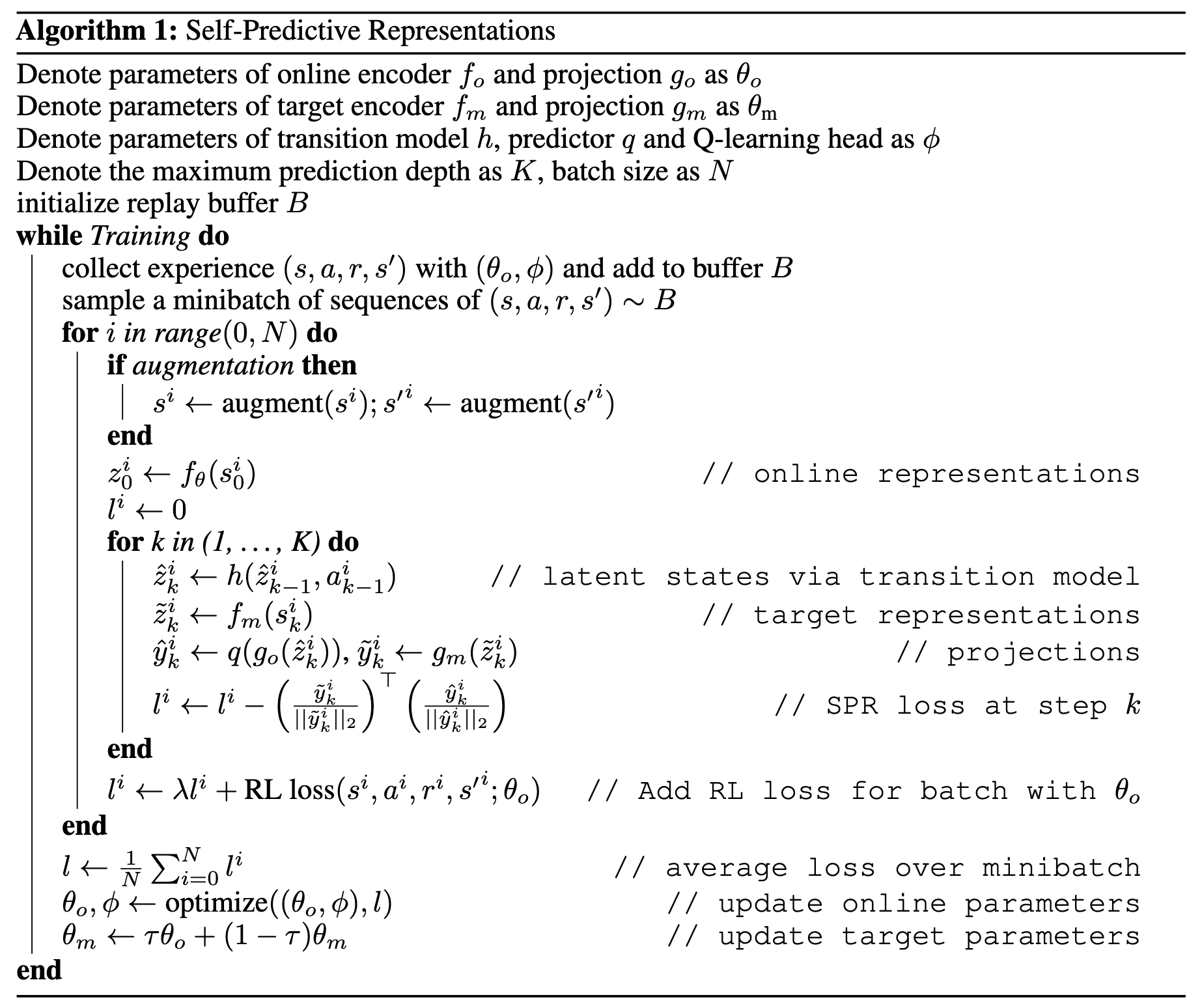
Let \((\mathbf{s}_{t:t+K}, \mathbf{a}_{t:t+K})\) denote a sequence of $K + 1$ previously experienced states and actions sampled from replay buffer $\mathcal{B}$ ($k = 5$ in practice). The SPR method consists of 4 main components:

1. Online & Target Networks $f_\mathrm{o}$, $f_\mathrm{m}$
   Analogous to popular self-supervised learning methods, the SPR framework has online network $f_\mathrm{o}$ and target network $f_\mathrm{m}$ to extract representations $\mathbf{z}_t$ from the observed states $\mathbf{s}_t$ with data augmentation. $$ \begin{aligned} \mathbf{z}_t & = f_\mathrm{o} (\mathbf{s}_t) \\ \tilde{\mathbf{z}}_t & = f_\mathrm{m} (\mathbf{s}_t) \end{aligned} $$ For each networks, each observation $\mathbf{s}_t$ independently augmented. Denoting the parameters of $f_\mathrm{o}$ as $\theta_\mathrm{o}$, those of $f_\mathrm{m}$ as $\theta_\mathrm{m}$, the update rule for $\theta_\mathrm{m}$ is EMA: $$ \theta_\mathrm{m} \leftarrow \tau \theta_\mathrm{m} + (1-\tau) \theta_\mathrm{o} $$ In practice, these encoders are implemented using he 3-layer convolutional encoder of DQN.
2. Transition Model $h$
   For the prediction objective, the SPR framework generates $K$ predictions $\mathbf{z}_{t+1:t+K}$ of future state representations $\tilde{\mathbf{z}}_{t+1:t+K}$ using an action-conditioned transition model $h$: $$ \begin{aligned} \mathbf{z}_{t+k+1} & = h (\mathbf{z}_{t+k}, \mathbf{a}_{t+k}) \\ \tilde{\mathbf{z}}_{t+k} & = f_\mathrm{m} (\mathbf{s}_{t+k}) \end{aligned} $$ starting from $\mathbf{z}_t = f_\mathrm{o} (\mathbf{s}_t)$.
3. Projection Heads $g_\mathrm{o}$, $g_\mathrm{m}$
   To avoid the loss of information in the representations extracted by encoders $f$, the projection heads $g_\mathrm{o}$ and $g_\mathrm{m}$ are attached that project online and target representations to a smaller latent space. Also, an additional prediction head $q$ to the online projections: $$ \begin{aligned} \mathbf{y}_{t+k} & = q (g_\mathrm{o} (\mathbf{z}_{t+k})) \\ \tilde{\mathbf{y}}_{t+k} & = g_\mathrm{m} (\tilde{\mathbf{z}}_{t+k}) \end{aligned} $$ The $g_\mathrm{m}$ parameters are also given by an EMA of the $g_\mathrm{o}$ parameters. In practice, the first layer of the DQN MLP head is reused as the SPR projection head.
4. Prediction Loss $\mathcal{L}_\theta^\texttt{SPR}$
   The future prediction loss for SPR is computed by summing over cosine similarities between the predicted and observed representations at timesteps $t + k$ for $1 \leq k \leq K$: $$ \mathcal{L}_\theta^\texttt{SPR} (\mathbf{s}_{t:t+K}, \mathbf{a}_{t:t+K}) = - \sum_{k=1}^K \left( \frac{\mathbf{y}_{t+k}}{\Vert \mathbf{y}_{t+k} \Vert_2 } \right)^\top \left( \frac{\tilde{\mathbf{y}}_{t+k}}{\Vert \tilde{\mathbf{y}}_{t+k} \Vert_2 } \right) $$ During training, the SPR loss is combined with the RL loss as an auxiliary loss, yielding the following full optimization objective: $$ \mathcal{L}_\theta^\texttt{total} = \mathcal{L}_\theta^\texttt{RL} + \lambda \mathcal{L}_\theta^\texttt{SPR} $$ Here, the SPR loss affects $f_\mathrm{o}$, $g_\mathrm{o}$, $q$, and $h$ and the RL loss affects $f_\mathrm{o}$ and the additional head attached to the encoder for the RL algorithm (e.g., in Rainbow, Q-learning head to estimate the Q-value from $\mathbf{z}$). In practice, the calculation of the SPR loss at episode boundaries are truncated to avoid encoding environment reset dynamics into the model.

$\mathbf{Fig\ 6.}$ The pseudocode of SPR (Schwarzer et al. 2021)

Experimental Results

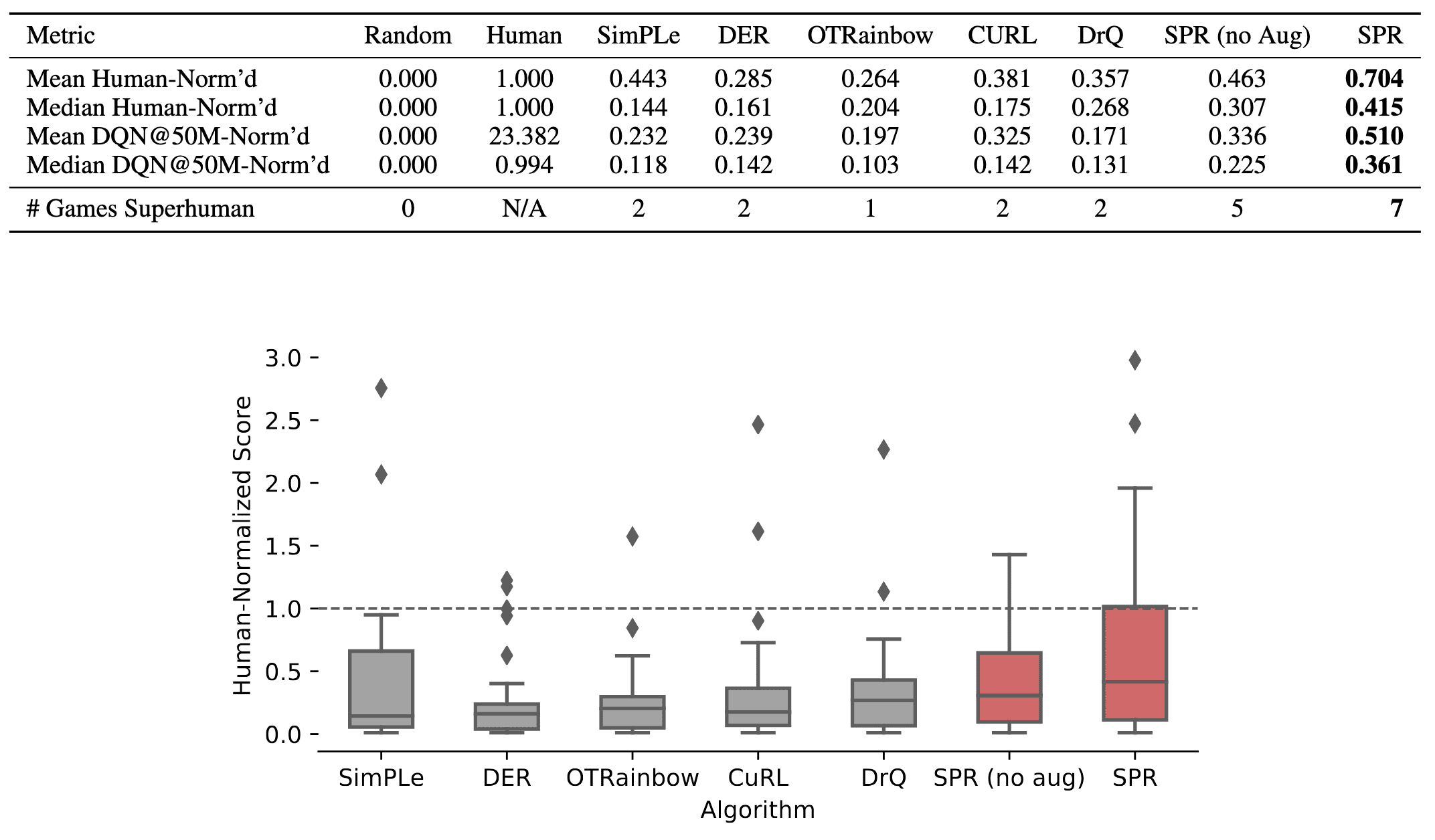
When combined with data augmentation, SPR attains a median human-normalized score of $0.415$, setting a state-of-the-art result fpr Atari-$100\mathrm{k}$ tasks. Also, SPR exhibits super-human performance on seven games within this data-limited setting: Boxing, Krull, Kangaroo, Road Runner, James Bond and Crazy Climber, surpassing the maximum of two achieved by any prior methods.

$\mathbf{Fig\ 7.}$ Performance of different methods on the Atari after $100\mathrm{k}$ environment steps (Schwarzer et al. 2021)

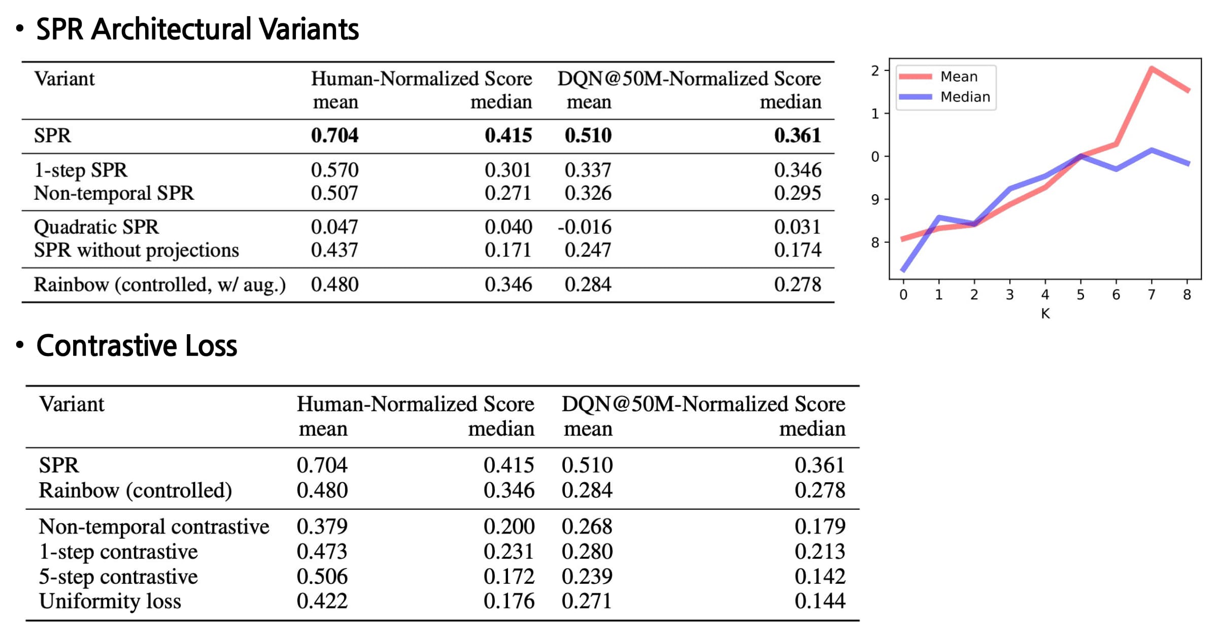
In addition, the ablations on SPR method provides several insights:

• Dynamics modeling is key
  A key distinction between SPR and other approaches is the incorporation of an explicit multi-step dynamics model. The authors demonstrate that extended dynamics modeling consistently enhances performance up to approximately $K=5$.
• Comparison with contrastive losses
  Although many recent works in representation learning utilize contrastive learning, the authors found that SPR consistently outperforms both temporal and non-temporal variants of contrastive losses. Additionally, employing a quadratic loss leads to representation collapse.
• Projections are critical
  SPR without projection and prediction heads has inferior performance, potentially because the effects of SPR in enforcing invariance to augmentation may be undesirable. The convolutional feature map, produced by only three layers, limits the ability to learn features that are both rich and invariant. Moreover, the convolutional network comprises only a small fraction of the capacity of SPR’s network, containing around 80,000 parameters out of a total of three to four million. By employing the first layer of the DQN head as a projection, the SPR objective can influence a much larger portion of the network, whereas its impact is restricted in this variant.

$\mathbf{Fig\ 8.}$ Ablation Studies on SPR (Schwarzer et al. 2021)

References

[1] Ni et al., “Bridging State and History Representations: Understanding Self-Predictive RL”, ICLR 2024
[2] Li et al., “Towards a Unified Theory of State Abstraction for MDPs”, AIandM 2022
[3] Schwarzer et al., “Data-Efficient Reinforcement Learning with Self-Predictive Representations”, ICLR 2021