[RL] TD7

In the field of reinforcement learning (RL), representation learning has proven effective for complex image-based tasks, yet it is frequently neglected in environments with low-level states, such as physical control problems. Fujimoto et al. NeurIPS 2023 introduces SALE, a novel approach for learning embeddings that capture the intricate interaction between state and action, enabling effective representation learning from low-level states. Additionally, they integrated SALE with an adaptation of checkpoints for RL into TD3 to form the TD7 algorithm, which substantially outperforms existing continuous control algorithms.

Preliminary: Twin Delayed DDPG (TD3)

The Q-learning algorithm is known to suffer from the overestimation of the value function. This challenge persists in an actor-critic setting, especially with deterministic actor, and is thus possible to adversely impact the policy. Twin-Delayed Deep Deterministic policy gradient (TD3), proposed by Fujimoto et al., 2018 implemented several techniques on top of DDPG (i.e. deterministic $\pi_\theta$) to mitigate the overestimation of the value function.

$\mathbf{Fig\ 1.}$ Overestimation Bias in the value estimates of DDPG.
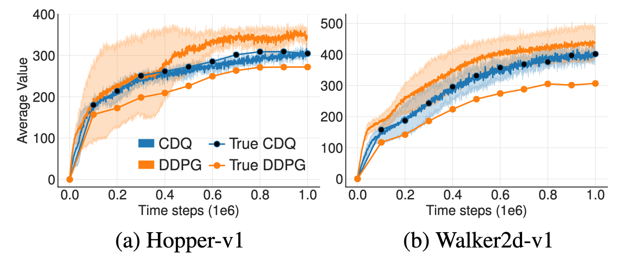
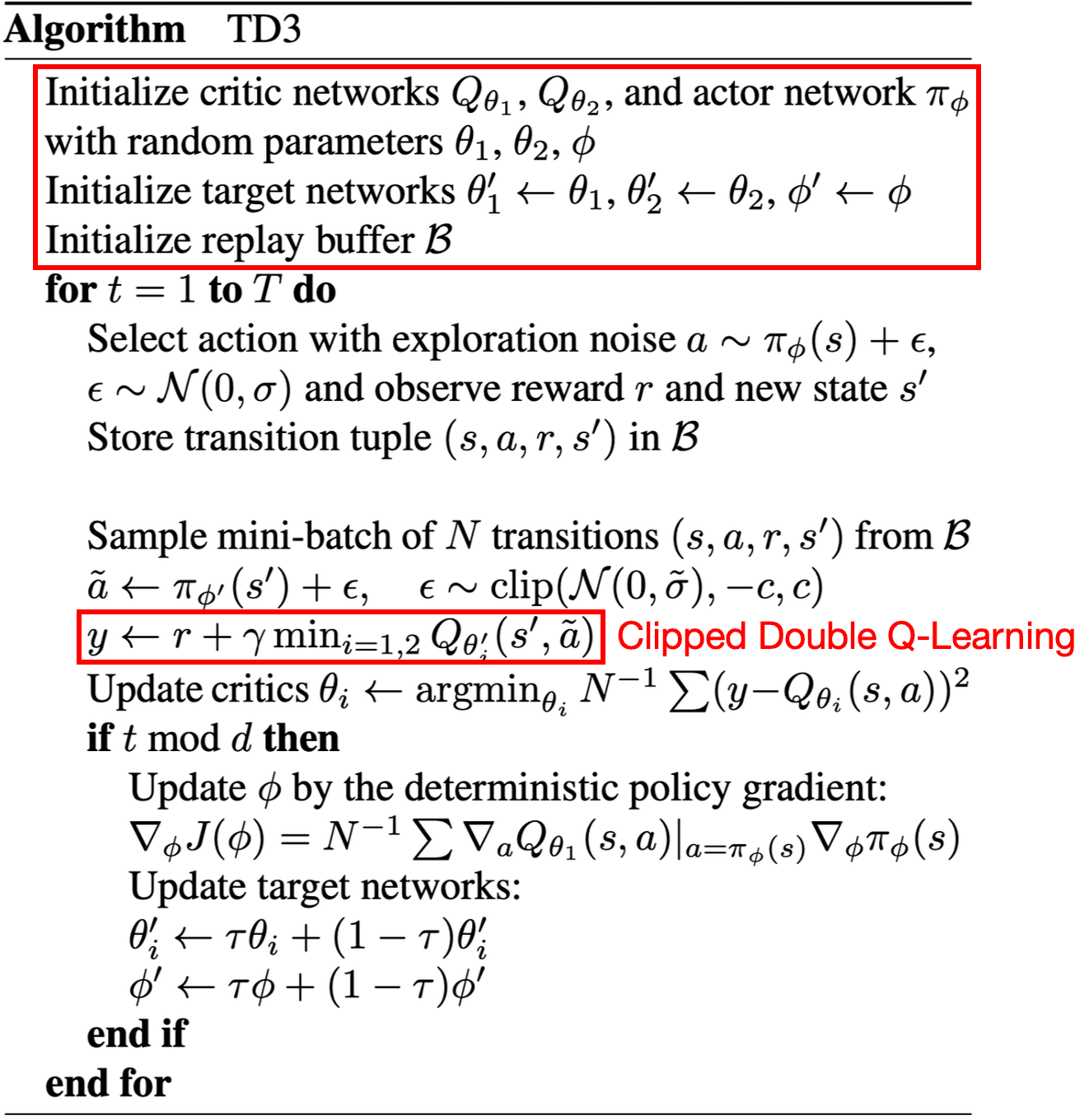
Proposed Clipped Double Q-learning (CDQ) of TD3 can effectively reduce such bias. (Fujimoto et al. 2018)

Motivation: Overoptimism of Q-Learning

Recall the update rule of Q-learning with estimated state-action value $Q$:

\[Q(\mathbf{s}, \mathbf{a}) \leftarrow Q(\mathbf{s}, \mathbf{a}) + \alpha \left[ r(\mathbf{s}, \mathbf{a}) + \gamma \underset{\mathbf{a}^\prime \in \mathcal{A}}{\max} Q (\mathbf{s}^\prime, \mathbf{a}^\prime) - Q(\mathbf{s}, \mathbf{a}) \right]\]

While this update will asymptotically approach the true optimal Q-value when $Q( \mathbf{s}, \mathbf{a})$ aligns with the true Q-value, it remains merely an estimation of the true Q-value. Consequently, the presence of noise in this estimation could impede the algorithm’s convergence to the true value. Indeed, Q-learning is known to incur a maximization bias-often referred to as overoptimism-the overestimation of the maximum expected action value. This issue was initially investigated by Thrun and Schwartz, 1993, wherein they theoretically demonstrated that if the action values contain random errors uniformly distributed in $[−\varepsilon, \varepsilon]$ then each target is overestimated up to $\gamma \varepsilon \frac{m−1}{m + 1}$ where $m$ is the number of actions.

The devil is in the $\max$ operator

The fundamental reason of the phenomenon lies in the $\max$ operator in the $Q$ target. As a consequence of function approximation noise, certain Q-values might be too small, while others might be excessively large. The $\max$ operator, however, always selects the largest value, rendering it especially sensitive to overestimations.

\[\underbrace{\mathbb{E} [\max ( Q_1, Q_2 )]}_{\text{What we are using}} \geq \underbrace{\max (\mathbb{E} [Q_1], \mathbb{E} [Q_2])}_{\text{What we want}}\]

To provide an intuitive understanding, consider the following example, borrowed from Ameet Deshpande’s post:

$\mathbf{Fig\ 2.}$ Environment for explanation (Ameet Deshpande)

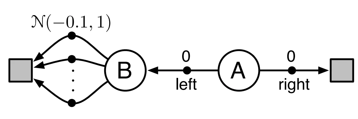
Suppose that the agent initially resides in state $\textrm{A}$ and if it selects the action $\textrm{right}$, it transitions to a terminal state and receives a reward of $0$. Conversely, if it selects the action $\textrm{left}$, it moves to state $\textrm{B}$, from which there exist numerous actions, each yielding rewards sampled from the Gaussian $\mathcal{N}(-0.1, 1)$, resulting in an expected reward of $-0.1$. In expectation, selecting the action $\textrm{right}$ appears advantageous due to the higher expected reward of $0$. However, the presence of reward variance gives rise to an unforeseen outcome.

Consider the scenario wherein the agent transitions to state $\textrm{B}$ and iteratively updates $Q$ by undergoing three trials, with two distinct actions $\mathbf{a}_1$ and $\mathbf{a}_2$ available at state $\textrm{B}$ for each trial, as outlined below:

	$Q(\textrm{A}, \textrm{left})$	$r(\textrm{B}, \mathbf{a}_1)$	$r(\textrm{B}, \mathbf{a}_2)$	$Q(\textrm{B}, \mathbf{a}_1)$	$Q(\textrm{B}, \mathbf{a}_2)$	$\underset{\mathbf{a} \in \mathcal{A}}{\max} Q(\textrm{B}, \mathbf{a})$
Trial 1	$0$	$-0.4$	$0.2$	$-0.2$	$0.1$	$0.1$
Trial 2	$0.05$	$-0.2$	$0.2$	$-0.2$	$0.2$	$0.2$
Trial 3	$0.125$	$0$	$-0.6$	$-0.1$	$-0.2$	$-0.1$
Trial 4	$0.0125$	-	-	-	-	-

As depicted in the table, despite $Q(\textrm{B}, \mathbf{a}_1)$ and $Q(\textrm{B}, \mathbf{a}_2)$ displaying negative values, the agent persistently chooses the $\textrm{left}$ action at state $\textrm{A}$. This behavior arises because the $\max$ operator exclusively neglect the negative value and optimistically selects the largest value.

Double Q-Learning

Therefore, the max operator in standard Q-learning (and DQN) uses the identical values both for action selection and evaluation, thus increasing the likelihood of selecting overestimated values and yielding overly optimistic value estimates. To mitigate this issue, we can simply decouple the selection from the evaluation, and such an approach is referred to as double Q-Learning proposed by [ 2010]. In double Q-Learning, two different Q-values $Q^A ( \cdot ; \boldsymbol{\theta}_A)$ and $Q^B ( \cdot ; \boldsymbol{\theta}_B)$ are learned by assigning each experience randomly to update one of the two Q-value functions. Consequently, the agent disentangles the selection and evaluation processes in Q-learning and revises its target as follows:

\[r (\mathbf{s}, \mathbf{a}) + \gamma \cdot Q (\mathbf{s}^\prime, \underset{\mathbf{a}^\prime \in \mathcal{A}}{\operatorname{arg max}} Q (\mathbf{s}^\prime, \mathbf{a}^\prime; \boldsymbol{\theta}); \boldsymbol{\theta}^\prime)\]

In this formulation, $Q^A$ is utilized for action selection, while $Q^B$ evaluates the chosen action with the Q target. And the roles of the two Q functions are randomly interchanged, as delineated in the following pseudocode:

$\mathbf{Fig\ 3.}$ The pseudocode for Double Q-Learning

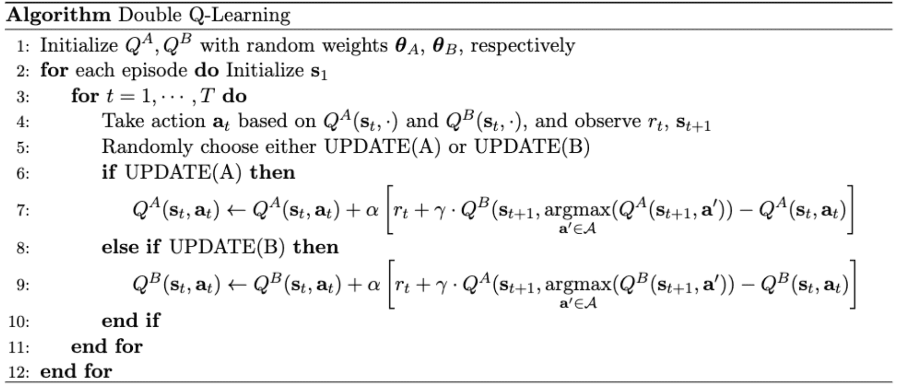
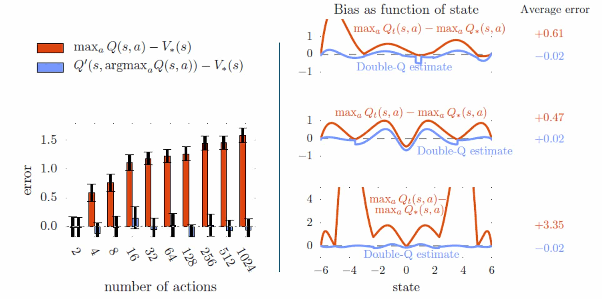
Consequently, double Q-learning is much robust to the overestimation regardless of the dimension of action space, while the overoptimism of the standard Q-learning increases with the number of actions as shown in the left part of figure below:

$\mathbf{Fig\ 4.}$ The overestimation comparison of the standard and double Q-learning (Hasselt et al., AAAI 2016)

Clipped Double Q-Learning

Recall that the $\max$ operator in standard Q-learning uses the identical values both for action selection and evaluation, thus increasing the likelihood of selecting overestimated values and yielding overly optimistic value estimates. And also recall that double Q-Learning learns two different Q-values $Q_{\phi_1}$ and $Q_{\phi_2}$ by assigning each experience randomly to update one of the two Q-value functions. Consequently, the agent can disentangles the selection and evaluation processes in Q-learning and revises its target as follows:

\[r (\mathbf{s}, \mathbf{a}) + \gamma \cdot Q (\mathbf{s}^\prime, \pi_{\phi} (\mathbf{s}^\prime); \phi^\prime) \text{ where } \pi_{\phi} (\mathbf{s}^\prime) = \underset{\mathbf{a}^\prime \in \mathcal{A}}{\arg\max} \; Q (\mathbf{s}^\prime, \mathbf{a}^\prime; \phi)\]

where $\phi$ and $\phi^\prime$ are randomly selected among $\phi_1$ and $\phi_2$. In actor-critic setting, this formulation is equivalent to the following Q target of a pair of critics $(Q_{\phi_1}, Q_{\phi_2})$ of which actors $(\pi_{\theta_1}, \pi_{\theta_2})$, with target critics $(Q_{\phi_1^\prime}, Q_{\phi_2^\prime})$:

\[\begin{aligned} \text{ Q-target of } Q_{\phi_1}: \quad & r (\mathbf{s}, \mathbf{a}) + \gamma Q_{\phi_2^\prime}(\mathbf{s}^\prime, \pi_{\theta_1}(\mathbf{s}^\prime))\\ \text{ Q-target of } Q_{\phi_2}: \quad & r (\mathbf{s}, \mathbf{a}) + \gamma Q_{\phi_1^\prime}(\mathbf{s}^\prime, \pi_{\theta_2}(\mathbf{s}^\prime)) \end{aligned}\]

Since two pairs are not entirely independent, due to the use of the opposite critic in the learning targets, as well as the same replay buffer, it is empirically demonstrated that it does not entirely eliminate the overestimation. Instead, clipped double Q-learning is simply implemented to be underestimated rather than overestimated:

\[\begin{aligned} & r (\mathbf{s}, \mathbf{a}) + \gamma \underset{n = 1, 2}{\min} Q_{\phi_n^\prime}(\mathbf{s}^\prime, \pi_{\theta_1^\prime}(\mathbf{s}^\prime))\\ & r (\mathbf{s}, \mathbf{a}) + \gamma \underset{n = 1, 2}{\min} Q_{\phi_n^\prime}(\mathbf{s}^\prime, \pi_{\theta_2^\prime}(\mathbf{s}^\prime)) \end{aligned}\]

While this update rule induces an underestimation bias, this is less likely to be propagated as underestimated actions will not be explicitly reinforced through the policy update. Additionally, in TD3, these update rules can be approximated with single actor $\pi_\theta$ optimized with respect to $Q_\phi$ for the sake of efficiency. If $Q_{\phi_1} > Q_{\phi_2}$, Q-target for both critics remains identical; otherwise, the Q-target is reduced similar to Double Q-learning framework.

$\mathbf{Fig\ 5.}$ Pseudocode for TD3: Clipped Double Q-Learning. (Fujimoto et al. 2018)

Delayed Target & Policy Updates

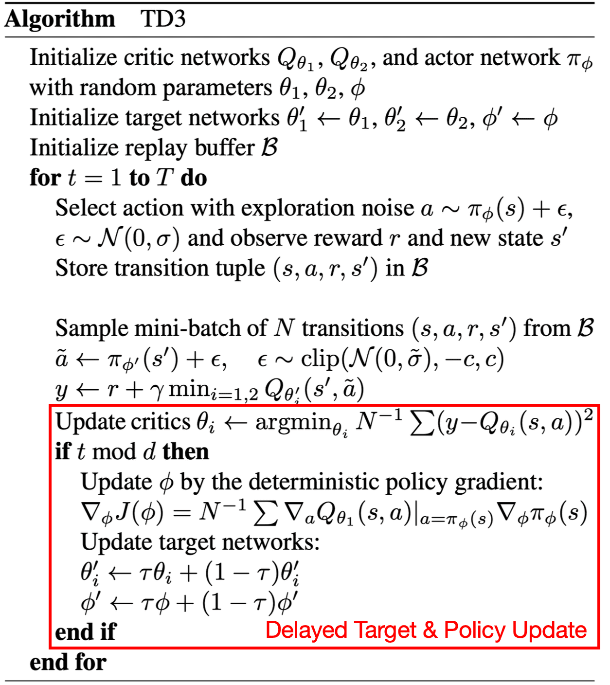
The authors observed that actor-critic methods can fail to learn due to the interplay between the actor and critic updates. Value estimates diverge through overestimation when the policy is poor, and the policy will become poor if the value estimate itself is inaccurate.

To avoid such divergent behaviors and further reduce the variance, TD3 proposed to slowly update the policy and target networks of DDPG after a fixed number of updates $d$ to the critic. This is analogous to the slow update of target networks in DQN frameworks.

$\mathbf{Fig\ 6.}$ Pseudocode for TD3: Delayed Target and Policy Updates. (Fujimoto et al. 2018)

Target Policy Smoothing

When updating the critic, a learning target using a deterministic policy is highly susceptible to inaccuracies induced by function approximation error, increasing the variance of the target. Furthermore, deterministic policies can easily overfit to narrow peaks in the value function.

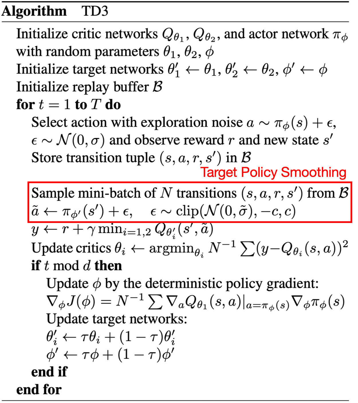
TD3 introduced a smoothing regularization strategy on the value function: adding a small amount of clipped random noises to the selected action and averaging over mini-batches:

\[\begin{gathered} y = r (\mathbf{s}, \mathbf{a}) + \gamma Q_{\phi^\prime} (\mathbf{s}^\prime, \pi_{\theta^\prime}(\mathbf{s}^\prime) + \epsilon) \\ \text{ where } \epsilon \sim \text{clip}(\mathcal{N}(0, \sigma), -c, +c) \end{gathered}\]

Fitting the value of narrow area around the target action offers the advantage of smoothing the value estimate by leveraging similar state-action value estimates. This approach enforces the idea that similar actions should yield similar values and mimics the expected update rule of expected SARSA:

\[\underbrace{y = r (\mathbf{s}, \mathbf{a}) + \gamma \mathbb{E}_{\mathbf{a}^\prime \sim \mu} \left[ Q (\mathbf{s}^\prime, \mathbf{a}^\prime) \right]}_{\text{Expected SARSA}} \Leftrightarrow \underbrace{y = r (\mathbf{s}, \mathbf{a}) + \gamma \mathbb{E}_{\epsilon} \left[ Q_{\phi^\prime} (\mathbf{s}^\prime, \pi_{\theta^\prime}(\mathbf{s}^\prime) + \epsilon) \right]}_{\text{TD3}}\]

$\mathbf{Fig\ 7.}$ Pseudocode for TD3: Target Policy Smoothing. (Fujimoto et al. 2018)

TD7

TD7 (TD3+4 additions) algorithm is a refined advancement of the TD3 algorithm, presented by Fujimoto et al. NeurIPS 2023. The authors demonstrated that TD7 substantially outperforms existing approaches, all while avoiding the added complexity found in competing methods, such as large ensembles, extra updates per time step, or environment-specific hyperparameters.

\[\begin{aligned} \textrm{TD7} = \textrm{TD3} & + \textrm{State-Action Learned Embedding (SALE)} \\ & + \textrm{Smarter Replay Buffer (LAP)} \\ & + \textrm{(for online) Policy Checkpoints} \\ & + \textrm{(for offline) BC Loss} \\ & + \textrm{Some other stuff} \\ \end{aligned}\]

SALE: State-Action Learned Embeddings

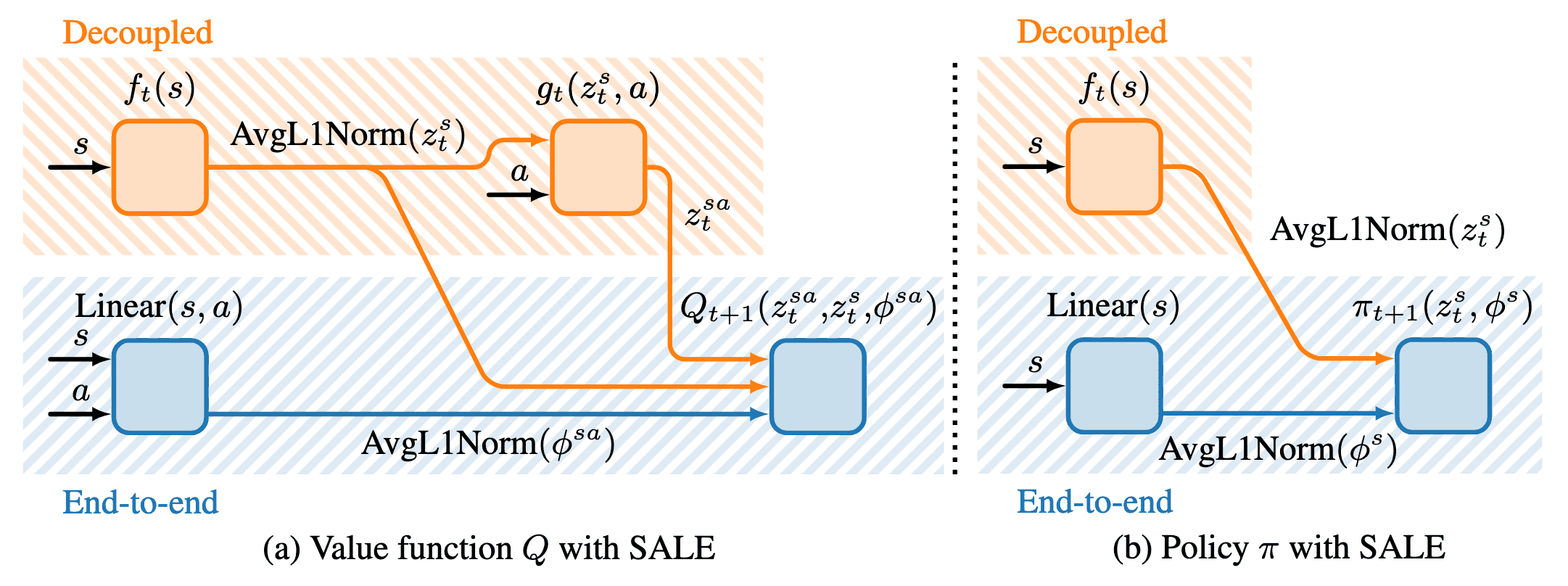
The core concept of TD7 lies in encoding state-action pairs into a latent space. This approach captures the intricate interplay and dynamics between state and action, enabling efficient representation learning, even when states are already at a low-level.

With state encoder $f$ and state-action encoder $g$, state-Action embedding $\mathbf{z}^{(\mathbf{s}, \mathbf{a})} = g(f(\mathbf{s}), \mathbf{a})$ aims to predict next state embedding $\mathbf{z}^{\mathbf{s}^\prime} = f (\mathbf{s}^\prime)$:

\[\mathcal{L} (f, g) := \left( g(f(\mathbf{s}), \mathbf{a}) - \texttt{stopgrad} (f (\mathbf{s}^\prime)) \right)^2 = \left( \mathbf{z}^{(\mathbf{s}, \mathbf{a})} - \texttt{stopgrad} (\mathbf{z}^{\mathbf{s}^\prime}) \right)^2\]

These learned embeddings are leveraged in main networks for Linear, $Q$, and policy $\pi$, but with stop gradient operator $\texttt{stopgrad}$:

\[\begin{aligned} Q(\mathbf{s}, \mathbf{a}) & \implies Q(\mathbf{z}^{(\mathbf{s}, \mathbf{a})}, \mathbf{z}^{\mathbf{s}}, \mathbf{s}, \mathbf{a}) \\ \pi (\mathbf{s}) & \implies \pi (\mathbf{z}^{\mathbf{s}}, \mathbf{s}) \end{aligned}\]

The encoders $(f, g)$ are trained online and concurrently with the RL agent (updated at the same frequency as the value function and policy), but are decoupled (gradients from the value function and policy are not propagated to $(f, g)$).

$\mathbf{Fig\ 8.}$ Diagram of SALE: State-Action Learned Embeddings (Fujimoto et al. 2023)

There are three additional details to the practical implemenation of SALE:

1. Normalized Embeddings: Keeping the embedding scale constant
   To prevent the monotonic growth and representation collapse, the AvgL1Norm, a normalization layer that divides the input vector by its average absolute value in each dimension is applied: $$ \texttt{AvgL1Norm} (\mathbf{x}) = \frac{\mathbf{x}}{\frac{1}{N} \sum_{i=1}^N \vert \mathbf{x}_i \vert} \text{ where } \mathbf{x} \in \mathbb{R}^N $$ This retains the relative scale of the embedding constant throughout training. $\texttt{AvgL1Norm}$ is applied to the state embedding and the state and action inputs (following a linear layer) to $Q$ and $\pi$, to keep them at a similar scale to the learned embeddings: $$ \begin{aligned} Q(\mathbf{z}^{(\mathbf{s}, \mathbf{a})}, \mathbf{z}^{\mathbf{s}}, \mathbf{s}, \mathbf{a}) & \implies Q(\mathbf{z}^{(\mathbf{s}, \mathbf{a})}, \texttt{AvgL1Norm}(\mathbf{z}^{\mathbf{s}}), \texttt{AvgL1Norm}(\texttt{Linear}(\mathbf{s}, \mathbf{a}))) \\ \pi (\mathbf{z}^{\mathbf{s}}, \mathbf{s}) & \implies \pi (\texttt{AvgL1Norm}(\mathbf{z}^{\mathbf{s}}), \texttt{AvgL1Norm}(\texttt{Linear}(\mathbf{s}))) \end{aligned} $$ It is worth noting that the AvgL1Norm is not applied on state-action embedding $\mathbf{z}^{(\mathbf{s}, \mathbf{a})}$, since it targets an already normalized embedding $\mathbf{z}^{\mathbf{s}^\prime}$.
2. Fixed Embeddings: Using target networks on embedding networks
   Similar to value targets, input embeddings also face a non-stationarity problem, where inconsistent inputs can lead to instability. To mitigate this, the embeddings used to train the current value and policy networks are frozen. Formally, at the iteration $t+1$, the input to the current $(Q_{t+1}, \pi_{t+1})$ uses embeddings $(\mathbf{z}_t^{(\mathbf{s}, \mathbf{a})}, \mathbf{z}_t^{\mathbf{s}})$ from the encoders $(f_t, g_t)$ at the previous iteration $t$: $$ \begin{aligned} Q_{t+1} (\mathbf{z}_t^{(\mathbf{s}, \mathbf{a})}, \mathbf{z}_t^\mathbf{s}, \mathbf{s}, \mathbf{a} ) & \approx r + \gamma Q_t (\mathbf{z}_{t-1}^{(\mathbf{s}^{\prime}, \mathbf{a}^{\prime})}, \mathbf{z}_{t-1}^{\mathbf{s}^{\prime}}, \mathbf{s}^{\prime}, \mathbf{a}^{\prime}), & & \text { where } \mathbf{a}^{\prime} \sim \pi_t(\mathbf{z}_{t-1}^{\mathbf{s}^{\prime}}, \mathbf{s}^{\prime}) \\ \pi_{t+1}(\mathbf{z}_t^\mathbf{s}, \mathbf{s}) & \approx \underset{\pi}{\arg \max} \; Q_{t+1}(\mathbf{z}_t^{(\mathbf{s}, \mathbf{a})}, \mathbf{z}_t^\mathbf{s}, \mathbf{s}, \mathbf{a}), & & \text { where } \mathbf{a} \sim \pi(\mathbf{z}_t^\mathbf{s}, \mathbf{s}) \end{aligned} $$ And every $n$ steps, the iteration is incremented and all target networks are updated simultaneously: $$ Q_t \leftarrow Q_{t+1}, \quad \pi_t \leftarrow \pi_{t+1}, \quad \left(f_{t-1}, g_{t-1} \right) \leftarrow \left(f_t, g_t \right), \quad \left(f_t, g_t \right) \leftarrow \left(f_{t+1}, g_{t+1}\right) $$
3. Clipped Values: Dealing with extrapolation error
   The use of learned embeddings led to abrupt spikes in value estimation, likely a result of action extrapolation from unseen state-action pairs. The following figure provides empirical evidence of this occurrence. Although performance trends upwards, significant dips in reward align with sharp jumps in the estimated value. It is evident that the dimension of $\mathbf{z}^{(\mathbf{s}, \mathbf{a})}$, as well as the state-action input, plays a crucial role in stabilizing value estimates. Moreover, increasing the input dimension, particularly when dependent on potentially unseen actions, can have a detrimental effect on stability.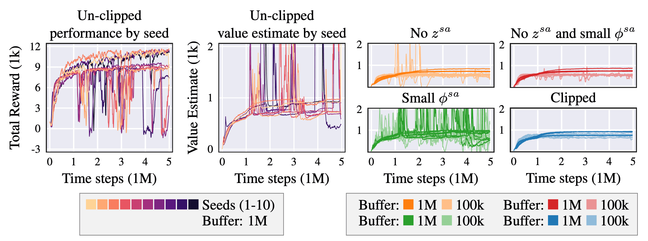

   

   $\mathbf{Fig\ 9.}$ Extrapolation error can occur in online RL when using state-action representation learning. $\phi^{(\mathbf{s}, \mathbf{a})}$ corresponds to $\texttt{Linear}(\mathbf{s}, \mathbf{a})$. Both embeddings and $\phi^{(\mathbf{s}, \mathbf{a})}$ have a default dimension size of $256$. Small $\phi^{(\mathbf{s}, \mathbf{a})}$ means that $\textrm{Dim}(\phi^{(\mathbf{s}, \mathbf{a})}) = 16$. No $\mathbf{z}^{(\mathbf{s}, \mathbf{a})}$ means the value function input is $Q(\mathbf{z}^\mathbf{s}, \mathbf{s}, \mathbf{a})$. The state embedding $\mathbf{z}^\mathbf{s}$ is left unchanged in all settings, showing that the state-action embedding $\mathbf{z}^{(\mathbf{s}, \mathbf{a})}$ and the linear layer over the state-action input $\phi^{(\mathbf{s}, \mathbf{a})}$ are the primary contributors to the extrapolation error. (Fujimoto et al. 2023)
   
   Luckily, in an online setting, this issue will be naturally corrected through feedback, so the key is to minimize its impact. To achieve this, the authors clip the target value into $\min$/$\max$ of previous Q-values, by tracking the range of values in the dataset $\mathcal{D}$, estimated over sampled mini-batches during training. $$ \begin{aligned} Q_{t+1} (\mathbf{z}_t^{(\mathbf{s}, \mathbf{a})}, \mathbf{z}_t^\mathbf{s}, \mathbf{s}, \mathbf{a} ) & \approx r + \gamma Q_t (\mathbf{z}_{t-1}^{(\mathbf{s}^{\prime}, \mathbf{a}^{\prime})}, \mathbf{z}_{t-1}^{\mathbf{s}^{\prime}}, \mathbf{s}^{\prime}, \mathbf{a}^{\prime}), \quad \text { where } \mathbf{a}^{\prime} \sim \pi_t(\mathbf{z}_{t-1}^{\mathbf{s}^{\prime}}, \mathbf{s}^{\prime}) \\ \implies Q_{t+1} (\mathbf{z}_t^{(\mathbf{s}, \mathbf{a})}, \mathbf{z}_t^\mathbf{s}, \mathbf{s}, \mathbf{a} ) & \approx r + \gamma \; \texttt{clip} \left( Q_t (\mathbf{z}_{t-1}^{(\mathbf{s}^{\prime}, \mathbf{a}^{\prime})}, \mathbf{z}_{t-1}^{\mathbf{s}^{\prime}}, \mathbf{s}^{\prime}, \mathbf{a}^{\prime}), \min_{(\mathbf{s}, \mathbf{a}) \in \mathcal{D}} Q_t (\mathbf{s}, \mathbf{a}), \max_{(\mathbf{s}, \mathbf{a}) \in \mathcal{D}} Q_t (\mathbf{s}, \mathbf{a}) \right) \\ \end{aligned} $$

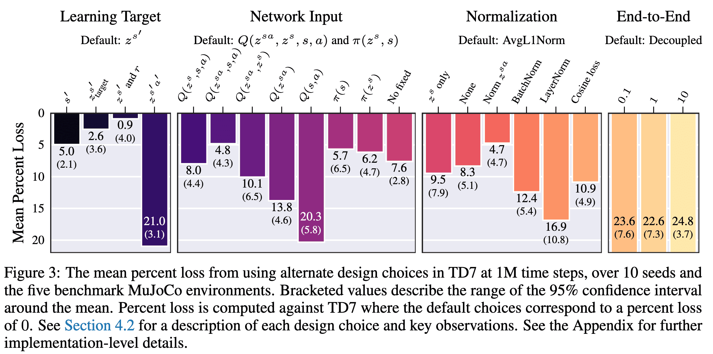
The following figure shows extensive experiments to verify their design choice; the mean percent loss of scores when modifying SALE in the TD7 algorithm.

$\mathbf{Fig\ 10.}$ The mean percent loss from using alternate design choices in TD7 at 1M time steps (Fujimoto et al. 2023)

LAP: Loss Adjusted PER

Recall that prioritized experience replay (PER) is a non-uniform sampling scheme for replay buffers where transitions are sampled by probability $p(i)$, proportional to their TD error $\delta (i)$ of a transition \(i = (\mathbf{s}, \mathbf{a}, r, \mathbf{s}^\prime)\):

\[p (i) = \frac{\vert \delta (i) \vert^\alpha}{\sum_{j} \vert \delta (i) \vert^\alpha}\]

where $\alpha$ is a hyperparameter that determines how much prioritization is used. To correct the int bias from PER that changes the training distribution, the value loss function with PER is also corrected by importance sampling:

\[\mathcal{L}_{\texttt{PER}}(\delta(i)) = w(i) \mathcal{L}(\delta(i)), \quad w(i)=\frac{\hat{w}(i)}{\max _j \hat{w}(j)}, \quad \hat{w}(i)=\left(\frac{1}{N} \cdot \frac{1}{p(i)}\right)^\beta\]

where $\beta$ is a hyperparameter that determines how much correction is used:

• $\beta=0$: no bias correction;
• $\beta=1$: no priority (uniform);

Fujimoto et al. NeurIPS 2020 provided theoretical framework to clarify the advantages of PER, by showing that any loss function computed with non-uniformly sampled data can be reformulated into an uniformly sampled loss function with the same expected gradient. Consequently, they introduced Loss-Adjusted Prioritized (LAP) experience replay, which simplifies PER by eliminating unnecessary importance sampling ratios and setting the minimum priority to be $1$. This approach systematically reduces bias and minimizes the occurrence of dead transitions with near-zero sampling probability.

Main theory: Any loss $\mathcal{L}_1$ with PER has an equivalent $\mathcal{L}_2$ without PER (in expectation)

First, consider that the expected gradient of a generic loss \(\mathcal{L}_1\) on the TD error $\delta(i)$ of transitions $i$ sampled by a distribution \(\mathcal{D}_1\) can be determined from another distribution \(\mathcal{D}_2\) by using the importance sampling ratio \(\frac{p_{\mathcal{D}_1} (i)}{p_{\mathcal{D}_2} (i)}\):

\[\underbrace{\mathbb{E}_{i \sim \mathcal{D}_1} \left[ \nabla_Q \mathcal{L}_1 (\delta (i)) \right]}_{\textrm{expected gradient of } \mathcal{L}_1 \textrm{ under } \mathcal{D}_1} = \mathbb{E}_{i \sim \mathcal{D}_2} \left[ \frac{p_{\mathcal{D}_1} (i)}{p_{\mathcal{D}_2} (i)} \nabla_Q \mathcal{L}_1 (\delta (i)) \right]\]

where the TD error with $i = (\mathbf{s}, \mathbf{a}, r, \mathbf{s}^\prime)$ is given by:

\[\delta (i) = Q_\theta (i) - y(i), \quad y(i) = r + \gamma Q_{\theta^\prime} (\mathbf{s}^\prime, \mathbf{a}^\prime)\]

Then, by introducing a second loss \(\mathcal{L}_2\) such that \(\nabla_Q \mathcal{L}_2 (\delta (i)) = \frac{p_{\mathcal{D}_1} (i)}{p_{\mathcal{D}_2} (i)} \nabla_Q \mathcal{L}_1 (\delta (i))\), the expected gradient of \(\mathcal{L}_1\) under \(\mathcal{D}_1\) and \(\mathcal{L}_2\) under \(\mathcal{D}_2\) would be equal:

\[\mathbb{E}_{i \sim \mathcal{D}_1} \left[ \nabla_Q \mathcal{L}_1 (\delta (i)) \right] = \mathbb{E}_{i \sim \mathcal{D}_2} \left[ \nabla_Q \mathcal{L}_2 (\delta (i)) \right]\]

That is, if we define \(\mathcal{D}_1\) to be the uniform distribution over a finite dataset $\mathcal{B}$ with $N = \vert \mathcal{B} \vert$ and \(\mathcal{D}_2\) be a prioritized sampling scheme \(p(i) = \frac{\vert \delta (i) \vert}{\sum_{j \in \mathcal{B}} \vert \delta (j) \vert}\), the importance sampling ratios used by PER can be absorbed into the loss function themselves, which gives an opportunity to simplify the algorithm. In practice, this relationship holds for MSE and \(\ell_1\) loss:

\[\mathbb{E}_{\mathcal{U}} \left[ \nabla_Q \mathcal{L}_\texttt{MSE} (\delta (i)) = \delta (i) \right] = \mathbb{E}_{\mathcal{D}_\texttt{PER}} \left[ \frac{\sum_{j \in \mathcal{B}} \delta(j)}{N \vert \delta (i) \vert} \delta(i) \right] \propto \mathbb{E}_{\mathcal{D}_\texttt{PER}} \left[ \texttt{sign} (\delta(i)) = \nabla_Q \mathcal{L}_{\ell_1} (\delta (i))\right]\]

In general, they revealed that a prioritized \(\mathcal{L}_\tau\) loss ($\tau > 0$) is roughly equivalent to a uniform \(\mathcal{L}_{\tau + \alpha - \alpha \beta}\) loss:

\[\begin{gathered} \mathcal{L}_{\mathcal{D}_\texttt{PER}}^\tau (\delta (i)) = w(i) \cdot \frac{1}{\tau} \vert \delta(i) \vert^\tau = \frac{\min_j \vert \delta (j) \vert^{\alpha \beta}}{\vert \delta (i) \vert^{\alpha \beta}} \cdot \frac{1}{\tau} \vert \delta(i) \vert^\tau \\ \Updownarrow \\ \mathcal{L}_\mathcal{U}^{\tau + \alpha - \alpha \beta} (\delta (i)) \propto \frac{\eta N}{\tau + \alpha - \alpha \beta} \vert \delta(i) \vert^{\tau + \alpha - \alpha \beta} \text{ where } \eta = \frac{\min_j \vert \delta (j) \vert^{\alpha \beta}}{\sum_j \vert \delta (j) \vert^\alpha} \end{gathered}\]

where $\alpha, \beta \in [0, 1]$ are the hyperparameters of PER. This point of view allows us to avoid any bias from weighted IS, and will reveal the problem of using prioritized $\mathcal{L}_2$ loss, which is what we often use.

The PER objective is biased if $\tau + \alpha − \alpha \beta \neq 2$

For better understanding of the prioritized $\mathcal{L}_2$ loss on the mirrored side to uniform buffer, consider the uniform $\mathcal{L}_1$ and $\mathcal{L}_2$ loss. Let $\mathcal{B}(\mathbf{s}, \mathbf{a}) \subset \mathcal{B}$ be the subset of transitions containing $(\mathbf{s}, \mathbf{a})$. In other words, for any \(i = (\mathbf{s}_i, \mathbf{a}_i, r_i, \mathbf{s}_i^\prime) \in \mathcal{B}(\mathbf{s}, \mathbf{a})\), \((\mathbf{s}_i, \mathbf{a}_i) = (\mathbf{s}, \mathbf{a})\). and $Q(i) = Q(\mathbf{s}, \mathbf{a})$. Then, each minimum of $\ell_1$ and $\ell_2$ loss provide the median and mean target:

\[\begin{aligned} \nabla_Q \mathbb{E}_{i \sim \mathcal{B}(\mathbf{s}, \mathbf{a})} \left[ \frac{1}{2} \delta(i)^2 \right] = 0 & \Rightarrow Q(\mathbf{s}, \mathbf{a}) = \texttt{mean}_{i \in \mathcal{B}(\mathbf{s}, \mathbf{a})} y(i) \\ \nabla_Q \mathbb{E}_{i \sim \mathcal{B}(\mathbf{s}, \mathbf{a})} \left[ \vert \delta(i) \vert \right] = 0 & \Rightarrow Q(\mathbf{s}, \mathbf{a}) = \texttt{median}_{i \in \mathcal{B}(\mathbf{s}, \mathbf{a})} y(i) \\ \end{aligned}\]

Observe that two losses have its own pros & cons:

• While the uniform \(\mathcal{L}_2\) provides an unbiased estimator of Q-target, going over the quadratic loss \(\mathcal{L}_{2 + \alpha - \alpha \beta}\) will be minimized by some expression which may favor outliers, as $2 + \alpha - \alpha \beta > 2$.
• Given the effects of function approximation and bootstrapping in deep reinforcement learning, one could argue the median is a reasonable loss function due to its robustness properties, but the gradient saturates at the optimal point.

Consequently, the appropriate choice of prioritized \(\mathcal{L}_\tau\) becomes to select $\tau$ to be $1 < \tau + \alpha - \alpha \beta \leq 2$, instead of $\tau = 2$ of which uniformly sampled loss function equivalent $\mathcal{L}_{2 + \alpha - \alpha \beta}$ provides a biased Q-target that favors high-error outliers. The authors proposed to use Huber loss with $\kappa = 1$, which swaps from \(\mathcal{L}_1\) to \(\mathcal{L}_2\) when the error falls below a threshold of $\kappa = 1$, scaling the appropriately gradient as $\delta(i)$ approaches $0$:

\[\mathcal{L}_{\texttt{Huber}}(\delta(i))= \begin{cases} 0.5 \delta(i)^2 & \text { if } \vert \delta(i) \vert\leq 1 \\ \vert \delta(i) \vert & \text { otherwise }\end{cases}\]

Since prioritized \(\mathcal{L}_2\) favors high-error outliers, we can clip all high-error samples to $1$:

\[p(i) = \frac{\max (\vert \delta (i) \vert^\alpha, 1)}{\sum_j \max (\vert \delta (j) \vert^\alpha, 1)}\]

Policy Checkpoints (for online RL)

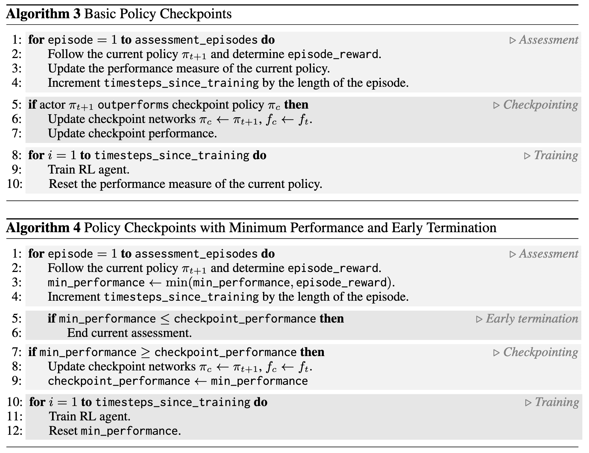
Deep RL algorithms are widely known for their inherent instability, which often results in significant variance in performance during training. To stabilize policy performance, the authors proposed using policy checkpoints, which obtained a high reward during training, in place of the current policy. They demonstrated that this could improve performance stability during testing.

$\mathbf{Fig\ 11.}$ Performance of individual seeds with and without checkpoints (Fujimoto et al. 2023)

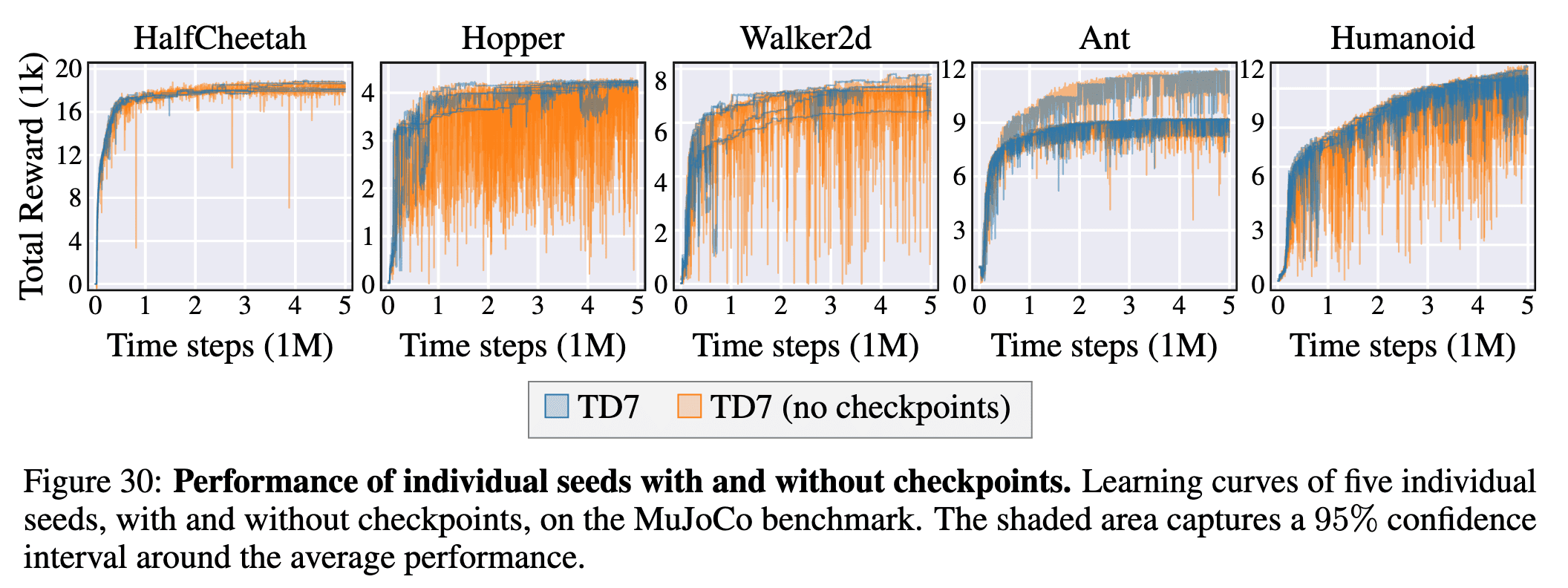
Much like many on-policy algorithms, TD7 maintains a fixed policy for several evaluation episodes, then batch the training that would have occurred.

• Standard off-policy RL: Collect a data point $\rightarrow$ train once.
• Proposed: Collect $N$ data points over several assessment episodes $\rightarrow$ train $N$ time;
  • Assess the current policy (using training episodes);
  • Train the current policy (with a number of time steps equal or proportional to the number of time steps viewed during assessment);
  • If the current policy outperforms the checkpoint policy, then update the checkpoint policy;

Note that checkpoints are not used in the offline setting, as there is no interaction with the environment. We further refine this approach:

1. Evaluate with minimum performance, not average.
   
   • Avoids policies that are unstable, even if they’re better on average.
   • This also allows us to prematurely halt the evaluation, if the minimum performance of the current policy drops below the minimum performance of the checkpoint, and move onto the next policy.
2. Restrict evaluation to $1$ episode in early learning stage (~$750\mathrm{k}$ steps).
   
   • Early stage policies require more exploration and fast feedback.

With these additional strategies, policy checkpoint surprisingly works well, even with high number of evaluation episodes ($20+$).

$\mathbf{Fig\ 12.}$ Learning curves on the MuJoCo benchmark, varying the maximum number episodes that the policy is fixed for (Fujimoto et al. 2023)

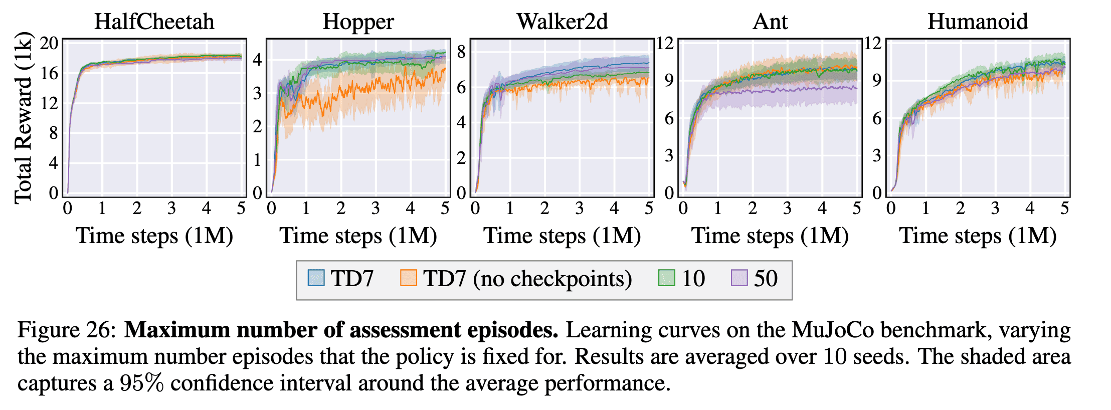
The following pseudocode summarizes the policy checkpoints of TD7:

$\mathbf{Fig\ 13.}$ The pseudocode of policy checkpoints (Fujimoto et al. 2023)

Behavior Cloning (for offline RL)

To make TD7 amenable to the offline RL setting, we add a behavior cloning loss to the policy update inspired by TD3+BC:

\[\begin{gathered} \pi \approx \underset{\pi}{\arg \max} \; \mathbb{E}_{(\mathbf{s}, \mathbf{a}) \sim \mathcal{D}}\left[ Q(\mathbf{s}, \pi(\mathbf{s}))-\lambda \cdot \color{red}{\texttt{stopgrad} (\mathbb{E}_{\mathbf{s} \sim \mathcal{D}}[Q(\mathbf{s}, \pi(\mathbf{s}))]) \times (\pi(\mathbf{s})- \mathbf{a})^2} \right] \\ \mathcal{L}\left(\pi_{t+1}\right) := - Q (\mathbf{s}, \pi (\mathbf{s})) + \lambda \cdot \color{red}{\texttt{stopgrad} (\mathbb{E}_{\mathbf{s} \sim \mathcal{D}}[Q (\mathbf{s}, \pi (\mathbf{s}))]) \times \left(\pi (\mathbf{s}) - \mathbf{a}\right)^2} \end{gathered}\]

where $\lambda = 0$ for the online setting. It is important to note that unlike original TD3+BC normalizes the Q value loss to match the scale between the two losses:

\[\begin{aligned} & \texttt{TD3}: && \pi = \underset{\pi}{\arg \max} \; \mathbb{E}_{(\mathbf{s}, \mathbf{a}) \sim \mathcal{D}} [Q (\mathbf{s}, \pi (\mathbf{s}))] \\ & \texttt{TD3+BC}: && \pi = \underset{\pi}{\arg \max} \; \mathbb{E}_{(\mathbf{s}, \mathbf{a}) \sim \mathcal{D}} [\color{red}{\lambda} Q (\mathbf{s}, \pi (\mathbf{s})) \color{red}{- (\pi (\mathbf{s}) - \mathbf{a})^2}] \text{ where } \lambda = \frac{\alpha}{\frac{1}{N} \sum_{(\mathbf{s}_n, \mathbf{a}_n)} Q(\mathbf{s}_n, \mathbf{a}_n)} \end{aligned}\]

TD7 upscales BC loss instead of downscaling Q loss.

Overall Algorithms

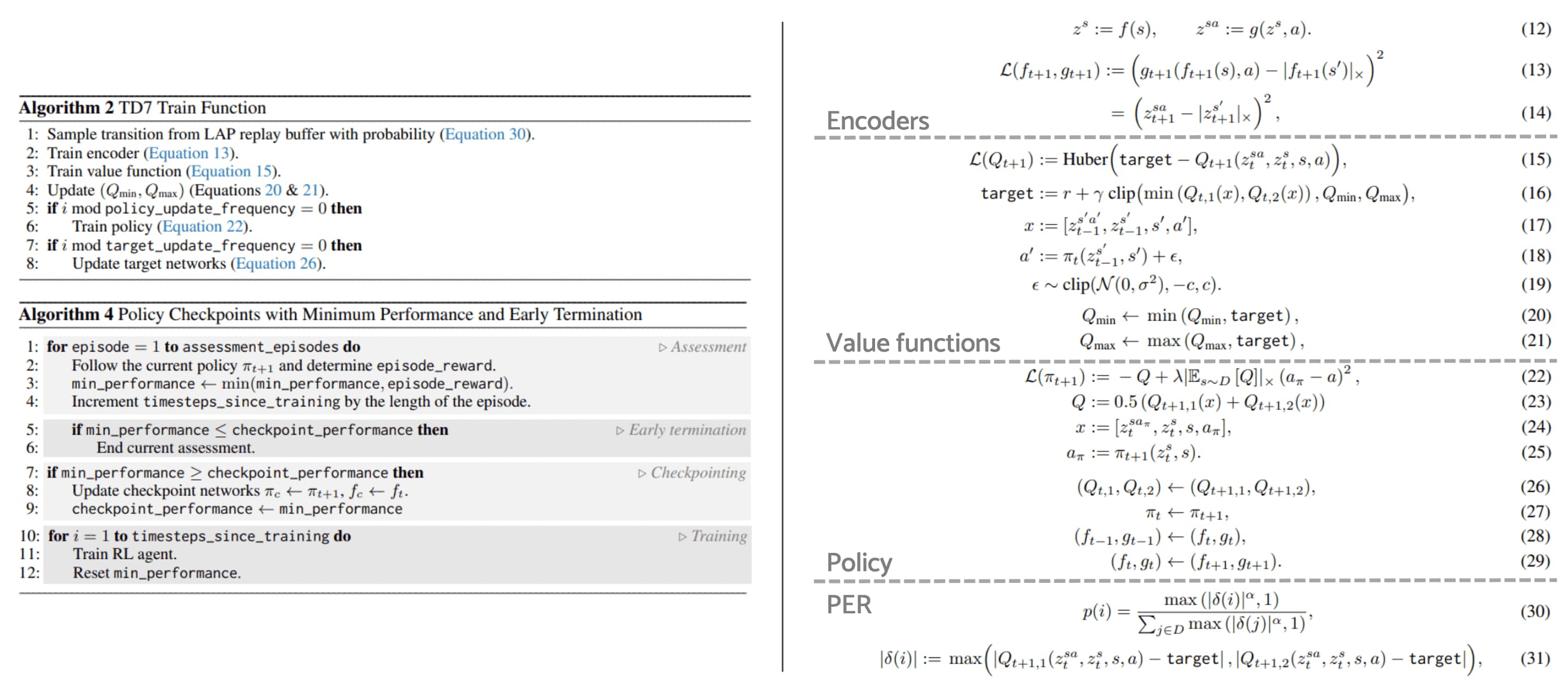
In summary, TD7 (TD3+4 additions) has several networks and sub-components:

• Two value functions $(Q_{t+1,1}, Q_{t+1,2})$
• Two target value functions $(Q_{t, 1}, Q_{t, 2})$
• A policy network $\pi_{t+1}$.
• A target policy network $\pi_t$.
• An encoder, with sub-components $(f_{t+1}, g_{t+1})$.
• A fixed encoder, with sub-components $(f_t, g_t)$.
• A target fixed encoder with sub-components $(f_{t−1}, g_{t−1})$.
• A checkpoint policy $\pi_c$ and checkpoint encoder $f_c$ ($g$ is not needed).

$\mathbf{Fig\ 14.}$ TD7 Algorithm (Fujimoto et al. 2023)

Encoder

The encoder is composed of two sub-networks $(f_{t+1} (\mathbf{s}), g_{t+1}) (\mathbf{z}^\mathbf{s}, \mathbf{a})$ where each network outputs an embedding:

\[\mathbf{z}^\mathbf{s} := f(\mathbf{s}) \quad \mathbf{z}^{(\mathbf{s}, \mathbf{a})} := g(\mathbf{z}^\mathbf{s}, \mathbf{a})\]

At each training step, the encoder is updated with the following loss:

\[\begin{aligned} \mathcal{L}(f_{t+1}, g_{t+1}) & := \left( g_{t+1} (f_{t+1} (\mathbf{s}), \mathbf{a}) - \texttt{stopgrad} (f_{t+1} (\mathbf{s}^\prime)) \right)^2 \\ & = \left( \mathbf{z}_{t+1}^{(\mathbf{s}, \mathbf{a})} - \texttt{stopgrad} (\mathbf{z}_{t+1}^{\mathbf{s}^\prime})\right)^2 \end{aligned}\]

Value function

TD7 uses a pair of value functions $(Q_{t+1,1}, Q_{t+1,2})$, as motivated by clipped double Q-learning of TD3, each taking input \([\mathbf{z}_{t-1}^{(\mathbf{s}^\prime, \mathbf{a}^\prime)}, \mathbf{z}_{t-1}^{\mathbf{s}^\prime}, \mathbf{s}^\prime, \mathbf{a}^\prime]\). At each training step, both value functions are updated with the following loss:

\[\begin{aligned} \mathcal{L} (Q_{t+1}) & := \texttt{Huber} \left( y_{t+1} - Q_{t+1} (\mathbf{z}_t^{(\mathbf{s}, \mathbf{a})}, \mathbf{z}_t^\mathbf{s}, \mathbf{s}, \mathbf{a} )\right) \\ y_{t+1} & := r (\mathbf{s}, \mathbf{a}) + \gamma \; \texttt{clip} \left( \min (Q_{t, 1} (\mathbf{x}), Q_{t,2} (\mathbf{x}))Q_{\min}, Q_{\max} \right) \\ \mathbf{x} & := \left[ \mathbf{z}_{t-1}^{(\mathbf{s}^\prime, \mathbf{a}^\prime)}, \mathbf{z}_{t-1}^{\mathbf{s}^\prime}, \mathbf{s}^\prime, \mathbf{a}^\prime \right] \\ \mathbf{a}^\prime & := \pi_t (\mathbf{z}_{t-1}^{\mathbf{s}^\prime}, \mathbf{s}^\prime) + \epsilon \\ \epsilon & \sim \texttt{clip} \left( \mathcal{N}(0, \sigma^2), -c, c \right) \end{aligned}\]

Taking the minimum of the value functions is from TD3’s Clipped Double Q-learning (CDQ). The use of Huber loss is in accordance to TD3 with the Loss-Adjusted Prioritized (LAP) experience replay. The next action $\mathbf{a}^\prime$ is sampled and clipped as TD3’s target policy smoothing. Note that the same embeddings \((\mathbf{z}_t^{(\mathbf{s}, \mathbf{a})}, \mathbf{z}_t^\mathbf{s})\) are used for each value function. And the $\texttt{clip}$ operation of target is proposed to deal with extrapolation error, where $Q_\min$ and $Q_\max$ are updated at each time step:

\[\begin{aligned} Q_{\min} & \leftarrow \min \left( Q_\min, y_{t+1} \right) \\ Q_{\max} & \leftarrow \max \left( Q_\max, y_{t+1} \right) \\ \end{aligned}\]

Policy

TD7 uses a single policy network which takes input $[\mathbf{z}^\mathbf{s}, \mathbf{s}]$. On every second training step (according to TD3’s delayed policy updates) the policy $\pi_{t+1}$ is updated with the following loss:

\[\begin{aligned} \mathcal{L} (\pi_{t+1}) & := -Q + \lambda \cdot \texttt{stopgrad} (\mathbb{E}_{\mathbf{s} \sim \mathcal{D}} [Q] ) \cdot (\mathbf{a}_\pi - \mathbf{a})^2 \\ Q & := \frac{1}{2} \left( Q_{t+1, 1} (\mathbf{z}_t^{(\mathbf{s}, \mathbf{a}_\pi)}, \mathbf{z}_t^\mathbf{s}, \mathbf{s}, \mathbf{a}_\pi) + Q_{t+1, 2} (\mathbf{z}_t^{(\mathbf{s}, \mathbf{a}_\pi)}, \mathbf{z}_t^\mathbf{s}, \mathbf{s}, \mathbf{a}_\pi) \right) \\ \mathbf{a}_\pi & := \pi_{t+1} (\mathbf{z}_t^\mathbf{s}, \mathbf{s}) \end{aligned}\]

The policy loss is the deterministic policy gradient (DPG) with a behavior cloning term to regularize as TD3+BC. Note that $\lambda = 0$ for online RL. After every $\texttt{target_update_freq}$ (250) training steps, the iteration is updated and each target (and fixed) network copies the network of the higher iteration:

\[\begin{aligned} (Q_{t,1}, Q_{t, 2}) & \leftarrow (Q_{t+1,1}, Q_{t+1, 2}) \\ \pi_t & \leftarrow \pi_{t+1} \\ (f_{t-1}, g_{t-1}) & \leftarrow (f_t, g_t) \\ (f_t, g_t) & \leftarrow (f_{t+1}, g_{t+1}) \end{aligned}\]

LAP

Gathered experience is stored in a replay buffer and sampled according to LAP, a prioritized replay buffer $\mathcal{D}$ where a transition tuple \(i := (\mathbf{s}, \mathbf{a}, r, \mathbf{s}^\prime)\) is sampled with probability:

\[\begin{aligned} p(i) & = \frac{\max (\vert \delta (i) \vert^\alpha, 1)}{\sum_{j \in \mathcal{D}} \max (\vert \delta (j) \vert^\alpha, 1)} \\ \vert \delta \vert & := \max \left( \vert Q_{t+1, 1} (\mathbf{z}_t^{(\mathbf{s}, \mathbf{a})}, \mathbf{z}_t^\mathbf{s}, \mathbf{s}, \mathbf{a}) - y_{t+1} \vert, \vert Q_{t+1, 2} (\mathbf{z}_t^{(\mathbf{s}, \mathbf{a})}, \mathbf{z}_t^\mathbf{s}, \mathbf{s}, \mathbf{a}) - y_{t+1} \vert \right) \end{aligned}\]

As suggested by Fujimoto et al. 2020, $\vert \delta (i) \vert$ is defined by the maximum absolute error of both value functions. The amount of prioritization used is controlled by a hyperparameter $\alpha$. New transitions are assigned the maximum priority of any sample in the replay buffer.

Experimental Results

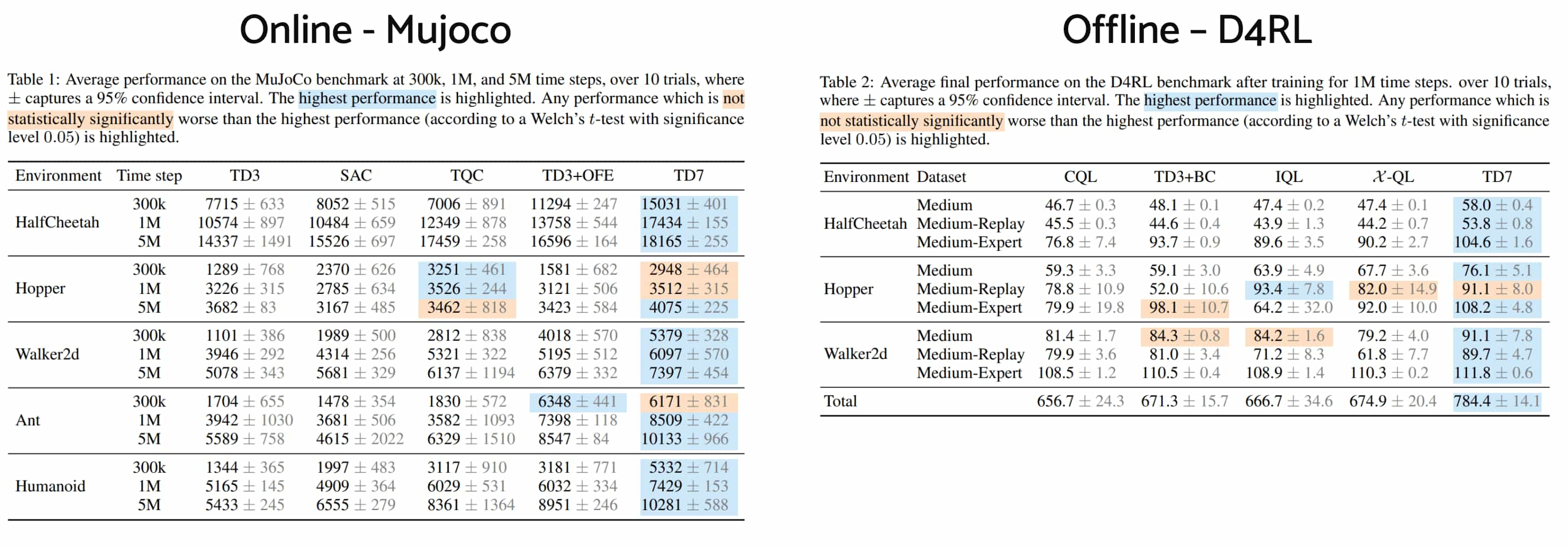
As a result, TD7 significantly match the performance of expensive offline algorithms and significantly outperform the state-of-the-art continuous control methods in both final performance and early learning.

$\mathbf{Fig\ 15.}$ Average performance on the online & offline RL benchmarks (Fujimoto et al. 2023)

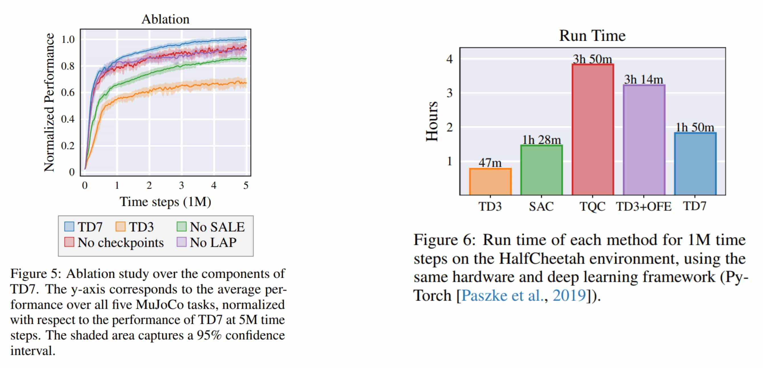
The results of an ablation study and the computational cost evaluations are reported in the following figure.

$\mathbf{Fig\ 16.}$ Ablation study & runtime evaluation (Fujimoto et al. 2023)

References

[1] Fujimoto et al., “Addressing Function Approximation Error in Actor-Critic Methods (TD3)”, ICML 2018
[2] Fujimoto et al., “A Minimalist Approach to Offline Reinforcement Learning (TD3+BC)”, NeurIPS 2021 Spotlight
[3] Fujimoto et al., “An Equivalence between Loss Functions and Non-Uniform Sampling in Experience Replay (LAP)”, NeurIPS 2020
[4] Fujimoto et al., “For SALE: State-Action Representation Learning for Deep Reinforcement Learning (TD7)”, NeurIPS 2023