[RL] Feature Discretization for RL

Much prior research has focused on learning representations with continuous features. However, discrete representations may offer a more natural fit for many modalities. For instance, language is inherently discrete, and speech is often represented as a sequence of symbols. Likewise, images can frequently be described succinctly using language. Moreover, discrete representations are well-suited for complex reasoning, planning, and predictive learning (e.g., “If it rains, I will use an umbrella”). And in practice, discrete prior recently shows remarkable success on various areas such as:

• DALL-E (text-image generative model) – image is encoded via VQ-VAE
• Many audio self-supervised learning method

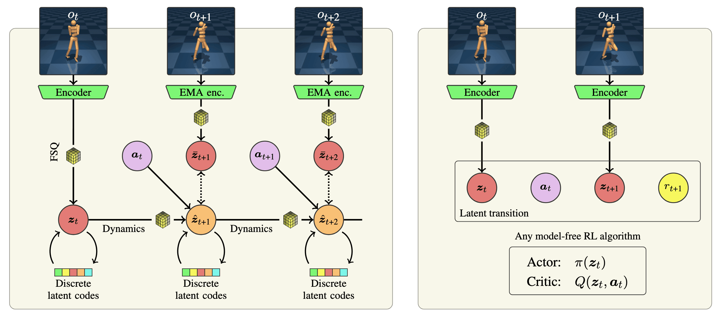
In response to this, several state-of-the-art RL algorithms employ feature discretization to enhance performance, sample-efficiency, and stability. This post explores the discretization techniques used in these RL algorithms, and presents a case study.

$\mathbf{Fig\ 1.}$ Example: Implicitly Quantized Representations (Scannell et al. 2024)

Discretization Techniques

Vector Quantizing VAE (VQ-VAE)

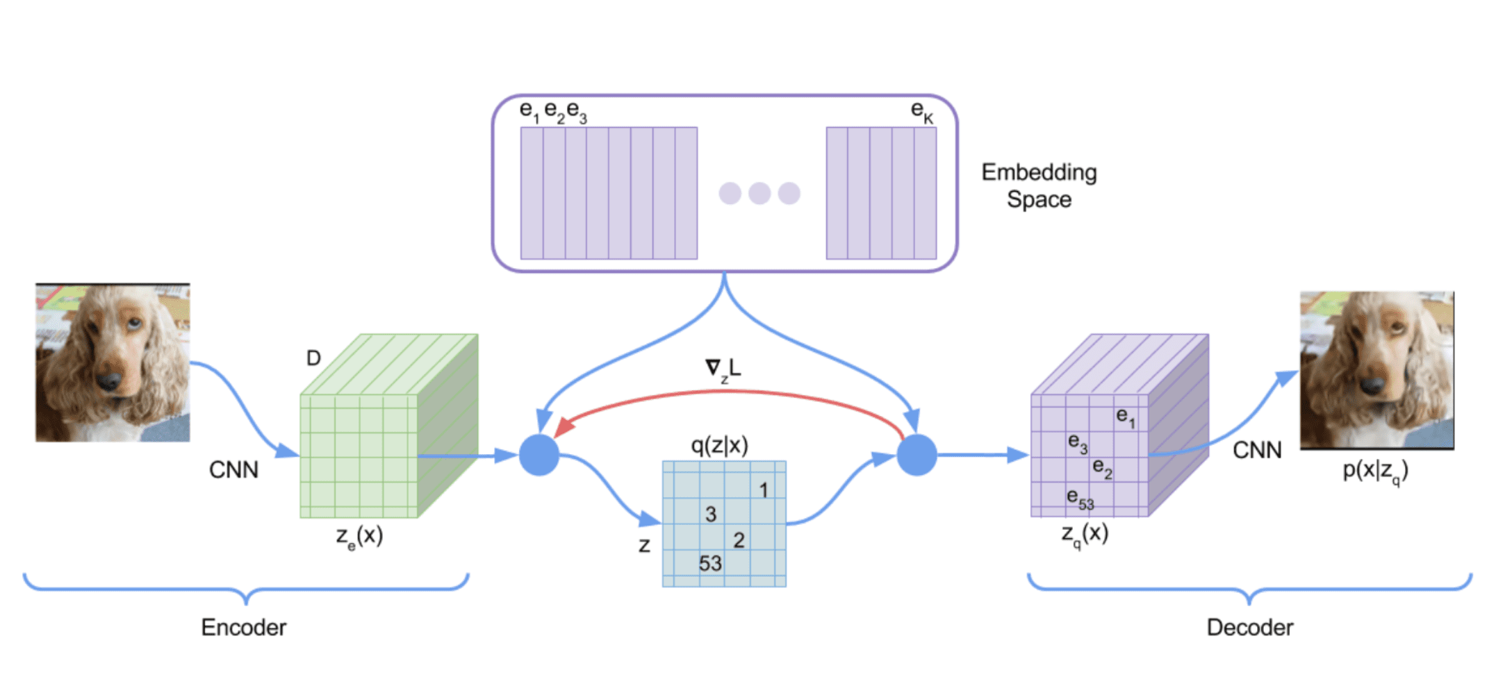
Despite the challenges associated with using discrete latent variables in deep learning, vector quantizing VAE (VQ-VAE) proposed by Van Den Oord et al. 2017 differentiably combines the VAE framework with discrete latent representations. The model is built on vector quantization (VQ) method, which maps $K$-dimensional vectors into a finite set of code vectors maintained in codebooks.

$\mathbf{Fig\ 2.}$ VQ-VAE framework (Van Den Oord et al. NeurIPS 2017)

Forward computation pipeline

Define a latent embedding space $\mathbf{e} \in \mathbb{R}^{K \times D}$, where $K$ is the size of the discrete latent space (i.e., a $K$-way categorical), and $D$ is the dimensionality of each latent embedding vector $\mathbf{e}_i$. Then, the forward computation of VQ-VAE operates as following:

1. An image input $\mathbf{x}$ is passed through an encoder $f_\theta$, producing output $f_\theta (\mathbf{x}) \in \mathbb{R}^D$. For brevity, assume $\mathbf{x} \in \mathbb{R}^N$ is one-dimensional vector.
2. The discrete latent variables $\mathbf{z}$ are then calculated by nearest neighbor look-up of the shared embedding space $\mathbf{e}$: $$ k = \arg \min_j \lVert f_\theta (\mathbf{x}) - \mathbf{e}_j \rVert_2 $$ Hence the posterior categorical distribution $q(\mathbf{z} \vert \mathbf{x})$ probabilities are defined as one-hot as follows: $$ \begin{aligned} q(\mathbf{z} = k \vert \mathbf{x}) = \begin{cases} 1 & \quad \text{for } k = \arg \min_j \arg \min_j \lVert f_\theta (\mathbf{x}) - \mathbf{e}_j \rVert_2 \\ 0 & \quad \text{ otherwise } \end{cases} \end{aligned} $$
3. The input $\mathbf{z}_\mathbf{q} (\mathbf{x})$ to the decoder $g_\phi$ is the corresponding embedding vector $\mathbf{e}_k$: $$ \begin{aligned} \mathbf{z}_\mathbf{q} (\mathbf{x}) = \mathbf{e}_k \quad \text{ where } \quad k = \arg \min_j \lVert f_\theta (\mathbf{x}) - \mathbf{e}_j \rVert_2 \end{aligned} $$

Although the above discussion is using an one-dimensional $\mathbf{x}$ and a single random variable $\mathbf{z}$ to represent the discrete latent variables, but it can be generalized to 2D matrix and tensors.

Training Loss

The training loss $\mathcal{L}$ has 3 components:

1. Reconstruction Loss
   From the reconstructed data $\tilde{\mathbf{x}} \sim p (\cdot \vert \mathbf{z}_\mathbf{q} (\mathbf{x}))$ from decoder output $\mathbf{z}_\mathbf{q} (\mathbf{x})$, the reconstruction loss encourages that the reconstruction $\tilde{\mathbf{x}}$ is close to the original $\mathbf{x}$: $$ \mathcal{L}_\texttt{recon} = \log p (\mathbf{x} \vert \mathbf{z}_\mathbf{q} (\mathbf{x})) $$ which is equivalent to $\ell_2$ loss $\Vert g_\phi (\mathbf{z}_\mathbf{q} (\mathbf{x})) - \mathbf{x} \Vert_2^2$ if the decoder distribution $p$ is set to be Gaussian distribution. Additionally, since the $\arg \min$ operator is not differentiable, the gradients $\nabla_\mathbf{z} \mathcal{L}$ from decoder input $\mathbf{z}_\mathbf{q} (\mathbf{x})$ is copied to the encoder output $f_\theta (\mathbf{x})$, which is called straight-through gradient estimation.
2. Vector Quantization Loss
   To learn embedding space $\mathbf{e}$, the vector quantization (VQ) loss is defined as $\ell_2$ error between the embedding space and the encoder outputs. Given a code vector $\mathbf{e}_i$, let $\{ \mathbf{z}_{i, j} \}_{j=1}^{n_i}$ be the set of encoder output vectors $f_\theta (\mathbf{x})$ that are quantized to $\mathbf{e}_i$. Then, the loss term is given by: $$ \mathcal{L}_{\texttt{VQ}} = \sum_{j=1}^{n_i} \Vert \texttt{stopgrad} ( \mathbf{z}_{i, j} ) - \mathbf{e}_i \Vert_2^2 $$ Note that it has a closed form solution (the average of elements in the set): $$ \mathbf{e}_i^* = \frac{1}{n_i} \sum_{j=1}^{n_i} \mathbf{z}_{i, j} $$ Therefore, instead of gradient descent, we can also use this update rule which is typically used in algorithms such as K-Means. However, we cannot use this update directly when working with minibatches since all $\{ \mathbf{z}_{i, } \}_{j=1}^{n_i}$ are not accessible. Instead, the embeddings are updated by exponential moving averages (EMA) as an online version of this update: $$ \begin{aligned} N_i^{(t)} & := \gamma N_{i}^{(t-1)} + (1-\gamma)n_i^{(t)} \\ m_i^{(t)} & := \gamma m_{i}^{(t-1)} + (1-\gamma) \sum_{j} z_{i, j}^{(t)} \\ e_i^{(t)} & := \frac{m_i^{(t)}}{N_i^{(t)}} \end{aligned} $$ where $\gamma \in [0, 1]$, and $N_i$ and $m_i$ are accumulated vector count and volume, respectively. (But the authors simply update the codebook with gradient descent in their official implementation, so you can ignore this.)
3. Commitment Loss
   Since there are no constraints on the embedding space, it can grow arbitrarily. A commitment loss, regularization to get encoder outputs and codebook close, is added to the overall loss function: $$ \mathcal{L}_{\texttt{commitment}} = \Vert f_\theta (\mathbf{x}) - \texttt{stopgrad} [ \mathbf{e} = \mathbf{z}_\mathbf{q} (\mathbf{x}) ] \Vert_2^2 $$ which encourages the encoder output $f_\theta (\mathbf{x})$ to stay close to the embedding space $\mathbf{e}$ and to prevent it from fluctuating too frequently from one code vector to another.

The following equation specifies the overall loss function.

\[\begin{aligned} \mathcal{L} & = \underbrace{\log p(\mathbf{x} \vert \mathbf{z}_\mathbf{q} (\mathbf{x}))}_{\textrm{reconstruction loss}} + \underbrace{\lVert \texttt{stopgrad}[\mathbf{z}_\mathbf{e} (\mathbf{x})] - \mathbf{e} \rVert_2^2}_{\textrm{VQ loss}} + \underbrace{\beta \times \lVert \mathbf{z}_\mathbf{e} (\mathbf{x}) - \texttt{stopgrad}[\mathbf{e}]\rVert_2^2}_{\textrm{commitment loss}} \\ & = \Vert g_\phi (\mathbf{z}_\mathbf{q} (\mathbf{x})) - \mathbf{x} \Vert_2^2 + \Vert \texttt{stopgrad} (f_\theta (\mathbf{x})) - \mathbf{z}_\mathbf{q} (\mathbf{x}) \Vert_2^2 + \beta \times \Vert f_\theta (\mathbf{x}) - \texttt{stopgrad} (\mathbf{z}_\mathbf{q} (\mathbf{x})) \Vert_2^2 \end{aligned}\]

where $\texttt{stopgrad}$ is the stop-gradient operator.

Straight-Through Estimator

For better understanding of straight-through estimator, let’s consider the following neural network that contains $\texttt{round}()$ function:

import torch
x = torch.tensor([1.1, 2.1], requires_grad=True)
y = 2*x
z = torch.round(y)
r = z.sum()

However, when we try to compute the gradient, we get a tensor of zeroes:

r 
# tensor(6., grad_fn=<SumBackward0>)
r.backward()
x.grad
# tensor([0., 0.])

This is because the rounding function has derivative zero almost everywhere.

$\mathbf{Fig\ 3.}$ The plot of $\texttt{round}$ function

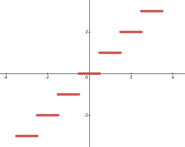
To circumvent this non-differentiability in order to maximize/minimize the output $r$, we could simply ignore the rounding function for the backpropagation and forcibly skip the gradient $\partial r / \partial z = \partial r / \partial y$ by PyTorch detach() method:

x = torch.tensor([1.1, 2.1], requires_grad=True)
y = 2*x
z = torch.round(y)
z = y + (z - y).detach() # Detach everything between z and y, including z
r = z.sum()

Then, we can get reasonable gradients of $x$ for our objective:

r 
# tensor(6., grad_fn=<SumBackward0>)
r.backward()
x.grad
# tensor([2., 2.])

When training VQ-VAE, the objective is to learn a codebook $\mathcal{C}$ whose elements create a compressed, semantic representation of the input data. During the forward pass, an image $\mathbf{x}$ is encoded into a representation $\mathbf{x}$ (usually a sequence of feature vectors), and each vector in $\mathbf{z}$ is quantized by replacing it with the nearest vector in $\mathcal{C}$.

As the quantization operation is non-differentiable, when training a VAE with VQ in the latent representation, the authors use the straight-through estimator, where gradients from the decoder input are copied to the encoder output, generating gradients for the encoder. Since this still does not produce gradients for the codebook vectors, they introduce two auxiliary losses to draw the codebook vectors towards the unquantized representation vectors, and vice versa.

Simplical Normalization (SimNorm)

Mostly studied in the sparse coding literature, overcomplete representations (representations of an input that are non-unique combinations of a number of basis vectors greater than the input’s dimensionality) with sparsity have been shown to enhance stability in noisy environments and yield more interpretable representations. Accordingly, Lavoie et al. ICLR 2023 proposed Simplicial Embeddings (SEM) in self-supervised learning methods, which are representations projected into $L$ simplices of $V$ dimensions each, using a $\texttt{softmax}$ operation. This method constrains the representation within a limited space during pre-training, introducing an inductive bias towards group sparsity.

Simplicial Embeddings (SEM)

In SEM, a representation \(\mathbf{z} \in \mathbb{R}^{LV}\) is splitted into $L$ vectors \(\mathbf{z}_i \in \mathbb{R}^N\) with $V$ dimensio. Then, vectors \(\mathbf{z}_i\) are normalized with the $\texttt{softmax}$ operation with temperature $\tau$, $\sigma_\tau$. These normalized vectors are concatenated into the vector \(\hat{\mathbf{z}}\). In this context, the softmax temperature $\tau$ plays a crucial role in regulating the inductive bias of SEM during pre-training: the lower the temperature, the stronger the bias towards sparsity.

$\mathbf{Fig\ 4.}$ Procedure to obtain Simplicial Embeddings (Lavoie et al. 2023)

The following pseudocode shows the simple PyTorch implementation of SEM:

def simnorm(z, V=8):
  shape = z.shape
  z = z.view(*shape[:-1], -1, V)
  z = softmax(z, dim=-1)
  return z.view(*shape)

SEM can be seamlessly integrated with any SSL methods by placing it between the encoder and the projector head. For instance, the following figure illustrates the incorporation of SEM into BYOL:

$\mathbf{Fig\ 5.}$ Integration of SEM awith BYOL (Lavoie et al. 2023)

Experimental Results

Applying SEM to seven different SSL methods, SEM increases the performance of linear probing on CIFAR-100.

$\mathbf{Fig\ 6.}$ Linear probe top-1 accuracy on CIFAR-100 trained for 1000 epochs with a ResNet-18 encoder (Lavoie et al. 2023)

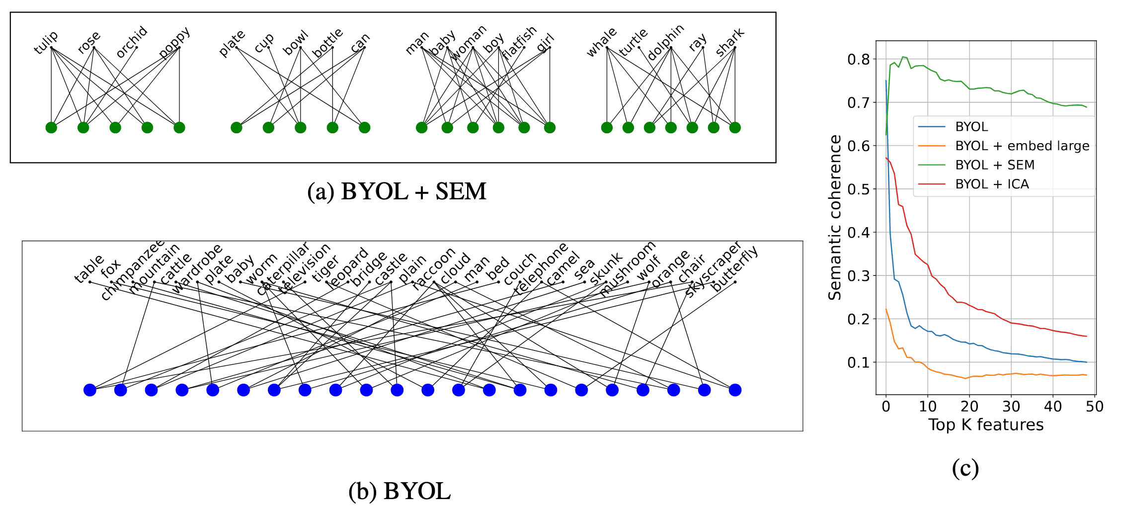
Interestingly, the features learned by SEM align coherently with the semantics in the training data. The authors visualize the most predictive features of a downstream linear classifier trained on CIFAR-100 and observe that classes with similar predictive features are semantically related. As a result, SEM demonstrates a high degree of coherence between the top $K$ features and the semantics of the super-classes in the CIFAR-100 categories.

$\mathbf{Fig\ 7.}$ Semantic coherence of the features (Lavoie et al. 2023)

Finite Scalar Quantization (FSQ)

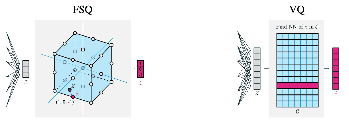
This VQ-VAE formulation, however, is challenging to optimize and leads to the well-documented issue of underutilized codebooks: as the size of $\mathcal{C}$ grows, many codewords remain unused. Mentzer et al. ICLR 2024 hypothesized that this arises from codebook collapse due to the movement of the codebook itself. To counter this, they proposed finite scalar quantization (FSQ), a simple fixed grid partition codebook.

$\mathbf{Fig\ 8.}$ FSQ v.s. VQ (Mentzer et al. 2024)

Finite Scalar Quantization

Given a $d$-dimensional representation $\mathbf{z} \in \mathbb{R}^d$, each dimension of $\mathbf{z}$ is bounded to $L$ values, and then $\texttt{round}$ to integers, resulting in the quantized $\hat{\mathbf{z}} \in \mathcal{C}$, the nearest point in this hypercube.

\[\begin{aligned} f(\mathbf{z}) & = \frac{L}{2} \times \tanh (\mathbf{z}) \in \left[ -\frac{L}{2}, \frac{L}{2} \right] \\ \hat{\mathbf{z}} & = \texttt{round}(f(\mathbf{z})) \end{aligned}\]

Therefore, $\vert \mathcal{C} \vert = L^d$. This exposition to the case where the $i$-th channel is mapped to $L_i$ values and get $\vert \mathcal{C} \vert = \prod_{i=1}^d L_i$. Again, the $\texttt{round}$ function is not differentiable, therefore this can be easily implemented using STE z_hat = f(z) + sg (round(f(z)) - f(z)). The following pseudocode shows the full PyTorch implementation of FSQ module:

class FSQ(Object)
  def __init__(self, levels: [8, 8, 8, 8], dim=512):
    levels = self.levels
    self.project_in = nn.Linear(dim, len(levels))
    self.project_out = nn.Linear(len(levels), dim)
  
  def forward(self, z):
    z = self.project_in(z)
    z = self.levels // 2 * nn.functional.tanh(z)
    z = z + (z.round() - z).detach()
    z = self.project_out(z)
    return z

Experimental Results

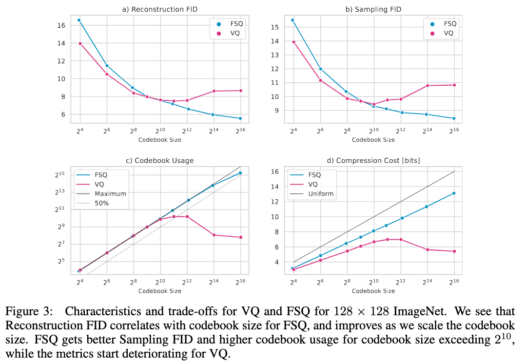
As a result, despite FSQ’s much simpler design, the authors achieved competitive performance across various vision tasks, indicating that FSQ avoids codebook collapse and eliminates the need for the complex mechanisms used in VQ (such as commitment losses, codebook reseeding, code splitting, and entropy penalties) to learn expressive discrete representations. Importantly, FSQ adheres to scalable laws: as the codebook size increases, FSQ’s reconstruction FID steadily improves. In contrast to VQ-VAE, where codebook usage diminishes with larger codebooks, FSQ’s usage continues to expand.

$\mathbf{Fig\ 9.}$ Characteristics and trade-offs for VQ and FSQ for $128 \times 128$ ImageNet (Mentzer et al. 2024)

RL Algorithms with Discretization

This section presents a case study on feature discretization in state-of-the-art RL algorithms. Specifically, the following three algorithms are the most notable examples:

• Dreamer V2 & V3 (VQ + SimNorm)
• TD-MPC2 (SimNorm)
• iQRL (FSQ)

Dreamer V2 & V3

Hafner et al. 2021 proposed DreamerV2 that supports the agent to learn purely from rollout data of the separately trained world model and firstly achieve human-level performance on $55$ Atari game tasks. Compared with the previous version (Dreamer), DreamerV2 replaces the Gaussian latent as proposed in PlaNet with the discrete latent, which brings superior performance. The possible reason for such effects would be the discrete latent representation can better fit the aggregate posterior and handle multi-modal cases.

Latent Dynamics Learning

The world model of DreamerV2 consists of an image encoder, a RSSM to learn the dynamics, and predictors for the image, reward, and discount factor. Note that the posterior state \(\mathbf{s}_t\) incorporates information about the current image \(\mathbf{o}_t\), while the prior state \(\hat{\mathbf{s}}_t\) aims to predict the posterior without access to the current image. Unlike in PlaNet and DreamerV1, the stochastic state of DreamerV2 is a vector of multiple categorical variables.

\[\begin{aligned}[t] & \text{Recurrent model:} && \mathbf{h}_t = \text{RNN}_\theta (\mathbf{h}_{t-1}, \mathbf{s}_{t-1}, \mathbf{a}_{t-1}) \\ & \text{Representation model:} && \mathbf{s}_t \sim \mathrm{q}_\theta (\mathbf{s}_t \vert \mathbf{h}_t, \mathbf{o}_t) \\ & \text{Transition predictor:} && \hat{\mathbf{s}}_t \sim \mathrm{p}_\theta (\hat{\mathbf{s}}_t \vert \mathbf{h}_t) \\ & \text{Image predictor:} && \hat{\mathbf{o}}_t \sim \mathrm{p}_\theta (\hat{\mathbf{o}}_t \vert \mathbf{h}_t, \mathbf{s}_t) \\ & \text{Reward predictor:} && \hat{r}_t \sim \mathrm{p}_\theta (\hat{r}_t \vert \mathbf{h}_t, \mathbf{s}_t) \\ & \text{Discount predictor:} && \hat{\gamma}_t \sim \mathrm{p}_\theta (\hat{\gamma}_t \vert \mathbf{h}_t, \mathbf{s}_t). \end{aligned}\] \[\mathcal{L}(\theta) = \mathbb{E}_{\mathrm{q}_{\theta} (\mathbf{s}_{1:T} \vert \mathbf{o}_{1:T}, \mathbf{a}_{1:T})} \left[ \sum_{t=1}^T \ln \mathrm{p}_\theta (\hat{\mathbf{o}}_t \vert \mathbf{h}_t, \mathbf{s}_t) + \ln \mathrm{p}_\theta (\hat{r}_t \vert \mathbf{h}_t, \mathbf{s}_t) + \ln \mathrm{p}_\theta (\hat{\gamma}_t \vert \mathbf{h}_t, \mathbf{s}_t) - \beta \cdot \text{KL}\left[ \mathrm{q}_\theta (\mathbf{s}_t \vert \mathbf{h}_t, \mathbf{o}_t) \Vert \mathrm{p}_\theta (\hat{\mathbf{s}}_t \vert \mathbf{h}_{t}) \right] \right]\]

where $\theta$ denotes their combined parameter vector and \(\mathrm{q}_{\theta} (\mathbf{s}_{1:T} \vert \mathbf{o}_{1:T}, \mathbf{a}_{1:T}) = \prod_{t=1}^T \mathrm{q}_{\theta} (\mathbf{s}_t \vert \mathbf{h}_t, \mathbf{o}_t)\).

$\mathbf{Fig\ 10.}$ World Model Learning of DreamerV2 (Hafner et al. 2021)

To optimize the discrete categorical latent states, straight-through gradients can be easily easy implemented via automatic differentiation.

$\mathbf{Fig\ 11.}$ Pseudocode of straight-through gradients. (Hafner et al. 2021)

For more details about Dreamer V2 & V3, please refer to my previous post.

TD-MPC2

To mitigate exploding gradients, TD-MPC2 proposed by Hafner et al. 2023 use the SEM (dubbed Simplicial Normalization (SimNorm) in the paper) of the latent representation $\mathbf{z}$, which projects $\mathbf{z} \in \mathbb{R}^{V \times L}$ into $L$ fixed-dimensional simplices using a softmax operation:

\[\texttt{SimNorm} (\mathbf{z}) = \texttt{concat}(\mathbf{g}_1, \cdots, \mathbf{g}_L)\]

where $V$ is the dimensionality of each simplex $\mathbf{g}$ constructed from $L$ partitions of $\mathbf{z}$ and:

\[\mathbf{g}_i = \texttt{softmax} (\mathbf{z}_{i: i + V}) = \frac{e^{\mathbf{z}_{i:i+V} / \tau}}{\sum_{j=1}^V e^{\mathbf{z}_{i:i+V, j} / \tau}}\]

$\mathbf{Fig\ 12.}$ The TD-MPC2 architecture (Hansen et al. 2024)

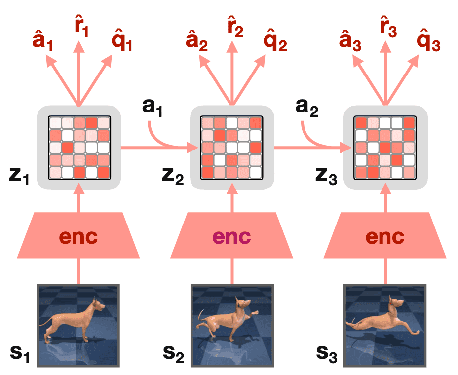
A significant advantage of embedding $\mathbf{z}$ as simplices is that it naturally biases the representation towards sparsity without enforcing hard constraints. Conceptually, it can be regarded as a “soft” version of the vector-of-categoricals method in VQ-VAE, analogous to how $\texttt{softmax}$ serves as a relaxation of the $\arg \max$ operator. While VQ-VAE encodes latent variables using a set of discrete codes ($L$ vector partitions each consisting of a one-hot encoding), SimNorm divides the latent state into $L$ vector partitions of continuous indices that each sum to $1$ with $\texttt{softmax}$.

Note that a temperature parameter $\tau \in [0, \infty]$ regulates the sparsity. For instance, $\tau \to \infty$ would concentrate all probability mass on individual categories, resulting in the discrete codes (one-hot encodings) in VQ-VAE. Conversely, $\tau = 0$ would produce trivial representations with uniform probability mass, prohibiting the propagation of information. Thus, SimNorm encourages sparsity in the representation without resorting to discrete codes or other rigid constraints.

$\mathbf{Fig\ 13.}$ VQ-VAE framework (Van Den Oord et al. NeurIPS 2017)

For more details about TD-MPC2, please refer to my previous post.

IQRL

In contrast to vision-based RL, learning a compact representation of an already compact state vector may seem unnecessary in state-based RL. However, task difficulty often arises from the complexity of the underlying transition dynamics rather than the observation space size. Thus, investigating representation learning for state-based RL is a promising research direction. Recently, self-supervised learning (SSL) approaches have achieved state-of-the-art results on continuous control benchmarks by developing robust representations with self-supervised losses.

However, these arpproaches are susceptible to representation collapse, where the encoder maps all observations to a constant latent representation. Consequently, it is common to pair the self-supervised latent-state consistency loss with additional terms, such as minimizing reward prediction error in the latent space. In response, IQRL by Scannell et al. 2024 utilized FSQ to prevent collapse by quantizing the latent representation without relying on any reconstruction loss.

Method components

IQRL has four main components:

\[\begin{aligned}[t] & \text{Encoder:} && \mathbf{z}_t = f (e_\theta (\mathbf{o}_t)) \\ & \text{Dynamics:} && \hat{\mathbf{z}}_{t+1} \sim f (\mathbf{z}_t + d_\phi (\mathbf{z}_t, \mathbf{a}_t)) \\ & \text{Value:} && q_t = q_\psi (\mathbf{z}_t, \mathbf{a}_t) \\ & \text{Policy:} && \mathbf{a}_t \sim \pi_\eta (\mathbf{z}_t) \end{aligned}\]

where $f$ is FSQ quantization:

\[\begin{aligned} f(\mathbf{z}) & = \frac{L}{2} \times \tanh (\mathbf{z}) \in \left[ -\frac{L}{2}, \frac{L}{2} \right] \\ \hat{\mathbf{z}} & = \texttt{round}(f(\mathbf{z})) \end{aligned}\]

$\mathbf{Fig\ 14.}$ IQRL Overview (Scannell et al. arXiv 2024)

Dynamics Loss

The encoders and dynamics are optimized through SSL objectives dubbed latent-state consistency loss:

\[\mathcal{L}_\texttt{rep} (\theta, \phi; \tau) = \sum_{n=0}^{H-1} \gamma_{\text{rep}}^n \left(\frac{f(\hat{\mathbf{z}}_{t+n} + d_{\phi}(\hat{\mathbf{z}}_{t+n}, \mathbf{a}_{t+n}))}{\Vert f(\hat{\mathbf{z}}_{t+n} + d_{\phi}(\hat{\mathbf{z}}_{t+n}, \mathbf{a}_{t+n})) \Vert_2}\right)^{\top} \left(\frac{f(e_{\bar{\theta}}(\mathbf{o}_{t+n+1}))}{\Vert f(e_{\bar{\theta}}(\mathbf{o}_{t+n+1}))\Vert_{2}} \right)\]

which minimizes the cosine similarity between the next state predicted by the dynamics model \(\hat{z}_{t+1} = f ( \hat{\mathbf{z}}_t + d_\phi( \hat{\mathbf{z}}_t, \mathbf{a}_t))\) and the next state predicted by the momentum encoder \(\bar{\mathbf{z}}_{t+1} = f (e_{\bar{\theta}} (\mathbf{o}_{t+1}))\) with $\bar{\theta} \leftarrow (1 − \tau) \bar{\theta} + \tau \theta$.

Model-Free RL Loss

The policy (actor) $\pi_\eta$ and action-value function (critic) $q_\psi$ can be learned by any model-free RL algorithms. The authors selected TD3 with $n$-step returns for optimizing critic:

\[\begin{aligned} \mathcal{L}_{q}(\psi; \tau) & = \mathbb{E}_{\tau \sim \mathcal{D}} \left[ \sum_{k=1}^{2} (q_{\psi_{k}}(f(e_\theta(\mathbf{o}_{t})), \mathbf{a}_{t}) - y)^{2} \right], \quad \forall k \in 1, 2 \\ \text{where } y &= \sum_{n=0}^{N-1} r_{t+n} + \gamma^{n} \min_{k \in \{1,2\}} q_{\bar{\psi}_{k}}(e_\theta(\mathbf{o}_{t+n+1}), \mathbf{a}_{t+n+1}) \quad \text{with} \; \mathbf{a}_{t+n} = \pi_{\bar{\eta}}(\mathbf{z}_{t+n}) + \epsilon_{t+n} \end{aligned}\]

where $\epsilon$ is a clipped Gaussian noise \(\epsilon_{t+n} \sim \texttt{clip} (\mathcal{N} (0, \sigma^2), −c, c)\) for target policy smoothing of TD3. Following TD3, the actor is learned by minimizing:

\[\mathcal{L}_{\pi}(\eta ; \tau) = - \mathbb{E}_{\mathbf{o}_{t} \sim \mathcal{D}} \left[ \min_{k\in \{1,2\} } q_{\psi_{k}}(\underbrace{f(e_{\theta}(\mathbf{o}_{t}))}_{\mathbf{z}_{t}}, \pi_{\eta}(f(e_{\theta}(\mathbf{o}_{t})))) \right]\]

in order to maximize the Q-value using the clipped double Q-learning trick to combat overestimation in Q-learning.

References

[1] Van Den Oord et al. “Neural discrete representation learning.” NeurIPS 2017.
[2] The official Tensorflow implementation of VQ-VAE
[3] AI StackExchange, “In VQ-VAE code what does this line of code signify?”
[4] Lavoie et al. “Simplicial Embeddings in Self-Supervised Learning and Downstream Classification”, ICLR 2023
[5] Mentzer et al. “Finite Scalar Quantization: VQ-VAE Made Simple”, ICLR 2024
[6] The official JAX implementation of FSQ
[7] Hafner et al. Mastering Atari with Discrete World Models., ICLR 2021
[8] Hafner et al. Mastering Diverse Domains through World Models., arXiv 2023
[9] Hansen et al. “TD-MPC2: Scalable, Robust World Models for Continuous Control”, ICLR 2024
[10] Scannell et al. “iQRL – Implicitly Quantized Representations for Sample-efficient Reinforcement Learning”, arXiv:2406.02696