[RL] Contrastive Visual RL

Developing agents capable of complex control tasks from high-dimensional observations, such as pixels, remains a challenge due to the sample inefficiency of reinforcement learning on raw pixel data. However, if state information is embedded within pixel data, then representations that capture relevant state information should, in principle, be learnable. Thus, with the right representation, learning from pixels could be as efficient as learning from state variables.

In computer vision, contrastive learning has become a powerful technique for learning effective representations, attributed to its capacity for deriving meaningful embeddings by contrasting similar and dissimilar data samples. In response, various visual RL approaches have incorporated self-supervised auxiliary tasks to enhance state representation learning, achieving notable progress. This post surveys visual RL research that utilizes the contrastive learning framework.

State Representation Learning

Contrastive Unsupervised Representations for RL (CURL)

CURL presented by Laskin et al. ICML 2020 is a general framework for combining contrastive learning with online RL setting. In CURL, a batch of transitions is sampled from the replay buffer. Observations are then data-augmented twice to form query and key observations, which are then encoded with the query encoder and key encoders, respectively. The queries are passed to the RL algorithm while query-key pairs are passed to the contrastive learning objective. During the gradient update step, only the query encoder is updated. The key encoder weights are the moving average (EMA) of the query weights similar to MoCo.

$\mathbf{Fig\ 1.}$ CURL Architecture (Laskin et al. 2020)

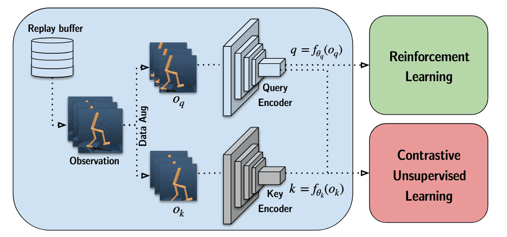
1. Query-Key Pair Generation
   Similar to self-supervised learning in the image setting, the anchor and positive observations are two different augmentations of the same image while negatives come from other images. CURL primarily relies on the random crop data augmentation, which is applied across the batch but consistently across each stack of frames to retain information about the temporal structure of the observation.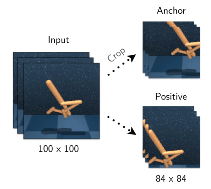

   
   

   $\mathbf{Fig\ 2.}$ Visually illustrating the process of generating an anchor and its positive using stochastic random crops (Laskin et al. 2020)
   
   Note that a significant difference between RL and computer vision settings is that an instance ingested by a model-free RL algorithm that operates from pixels is not just a single image but a stack of frames. This way, performing instance discrimination on frame stacks allows CURL to learn both spatial and temporal discriminative features.
2. Contrastive Loss
   For given augmented query observation $\mathbf{o}_q$ and key observation $\mathbf{o}_k$, CURL employs the bilinear inner product similarity for the InfoNCE loss: $$ \mathcal{L} = \log \frac{\exp (\mathbf{q}^\top \mathbf{W} \mathbf{k}_+)}{\exp (\mathbf{q}^\top \mathbf{W} \mathbf{k}_+) + \sum_{i=0}^{K - 1} \exp (\mathbf{q}^\top \mathbf{W} \mathbf{k}_i) } $$ where $\mathbf{W}$ is a learned parameter matrix and $\mathbf{o}_q$ and $\mathbf{o}_k$ are encoded by encoders $f_q$ and $f_k$: $$ \begin{aligned} \mathbf{q} & = f_q (\mathbf{o}_q) \\ \mathbf{k} & = f_q (\mathbf{o}_k) \\ \end{aligned} $$
3. Momentum Target Encoder
   Given $f_q$ parametrized by $\theta_q$ and $f_k$ parametrized by $\theta_k$, CURL performs the EMA update: $$ \theta_k \leftarrow m \cdot \theta_k + (1-m) \cdot \theta_q $$ and encodes any target $\mathbf{o}_k$ using $\texttt{stopgrad}(f_k(\mathbf{o}_k))$.

The following algorithm is the PyTorch-like pseudocode of CURL:

# f_q, f_k: encoder networks for anchor
# (query) and target (keys) respectively.
# loader: minibatch sampler from ReplayBuffer
# B-batch_size, C-channels, H,W-spatial_dims
# x : shape : [B, C, H, W]
# C = c * num_frames; c=3 (R/G/B) or 1 (gray)
# m: momentum, e.g. 0.95
# z_dim: latent dimension
f_k.params = f_q.params
W = rand(z_dim, z_dim) # bilinear product.
for x in loader: # load minibatch from buffer
  x_q = aug(x) # random augmentation
  x_k = aug(x) # different random augmentation
  z_q = f_q.forward(x_q)
  z_k = f_k.forward(x_k)
  z_k = z_k.detach() # stop gradient
  proj_k = matmul(W, z_k.T) # bilinear product
  logits = matmul(z_q, proj_k) # B x B
  # subtract max from logits for stability
  logits = logits - max(logits, axis=1)
  labels = arange(logits.shape[0])
  loss = CrossEntropyLoss(logits, labels)
  loss.backward()
  update(f_q.params) # Adam
  update(W) # Adam
  f_k.params = m * f_k.params + (1-m) * f_q.params

Experimental Results

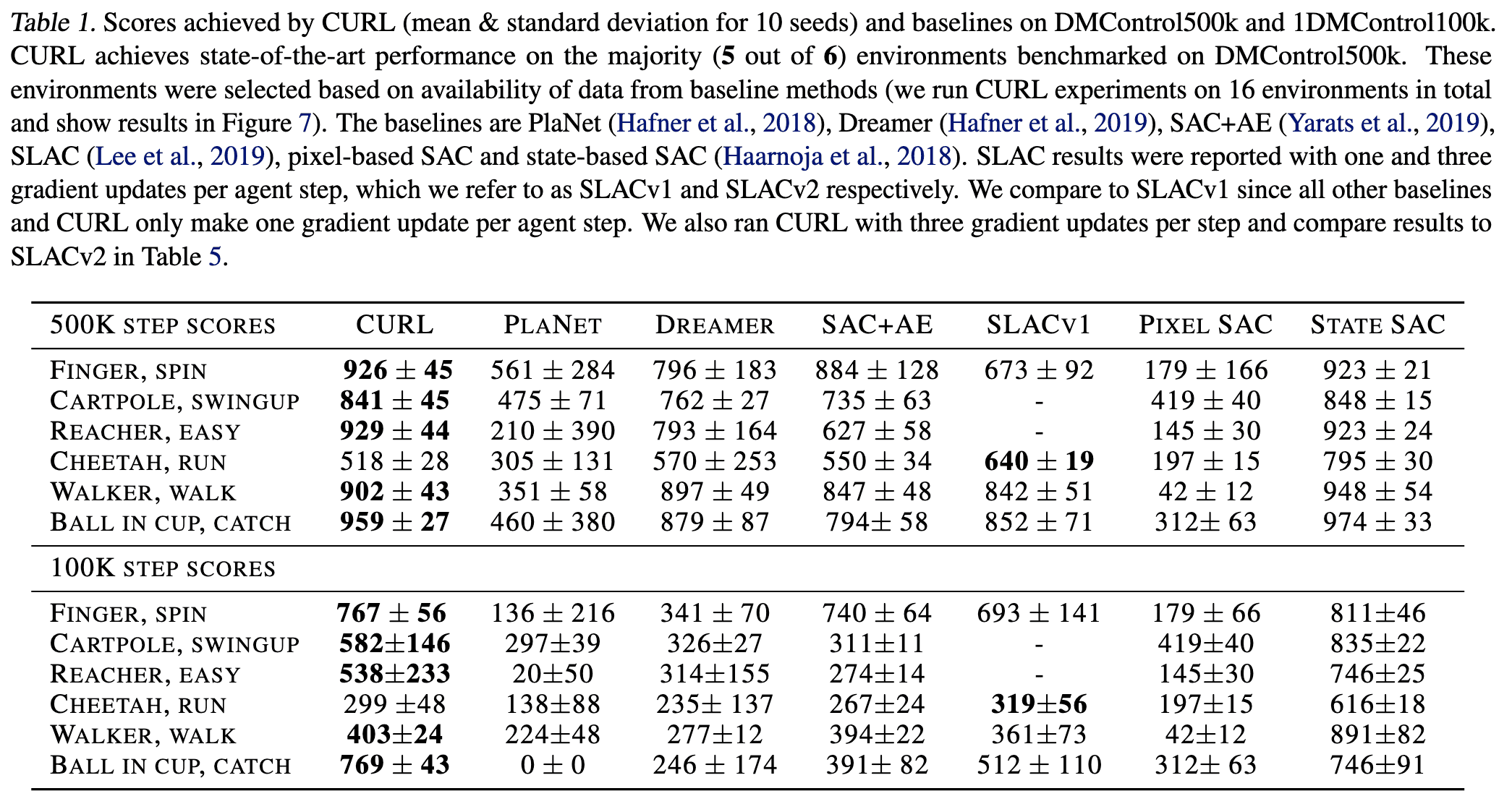
The performance of CURL on DMControl benchmarks is reported in the following table.

$\mathbf{Fig\ 3.}$ Scores achieved by CURL on DMControl benchmarks (Laskin et al. 2020)

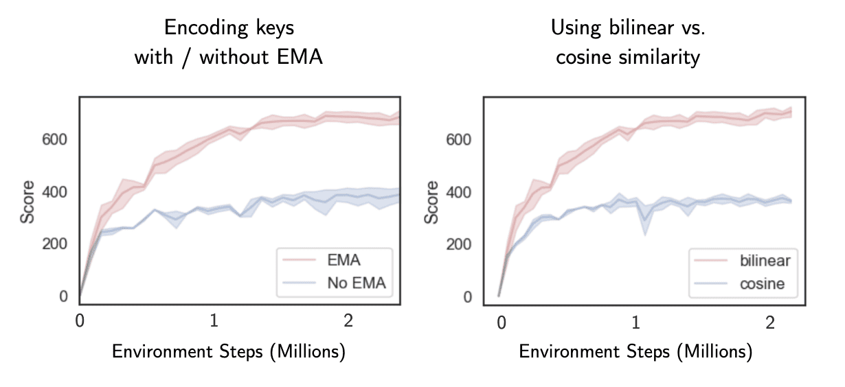
Notably, the bi-linear similarity measure outperforms the normalized dot-product used in state-of-the-art contrastive learning methods in computer vision such as MoCo and SimCLR.

$\mathbf{Fig\ 4.}$ Performance on cheetah-run environment ablated two-ways (Laskin et al. 2020)

Augmented Temporal Contrast (ATC)

Most visual representation learning in RL simultaneously learns visual features and a control policy in an end-to-end manner. While the simplicity of end-to-end approaches is appealing, depending on the reward function to learn visual features can be highly restrictive. For instance, this approach makes feature learning challenging under sparse rewards and may limit the generalizability of learned features to a single task.

Stooke et al. ICML 2021 investigated methods for learning visual representations that are independent of rewards without compromising control policy performance. They proposed Augmented Temporal Contrast (ATC) that decouples representation learning from RL, achieving performance comparable to or even exceeding that of end-to-end RL approaches.

$\mathbf{Fig\ 5.}$ Augmented Temporal Contrast (Stooke et al. 2020)

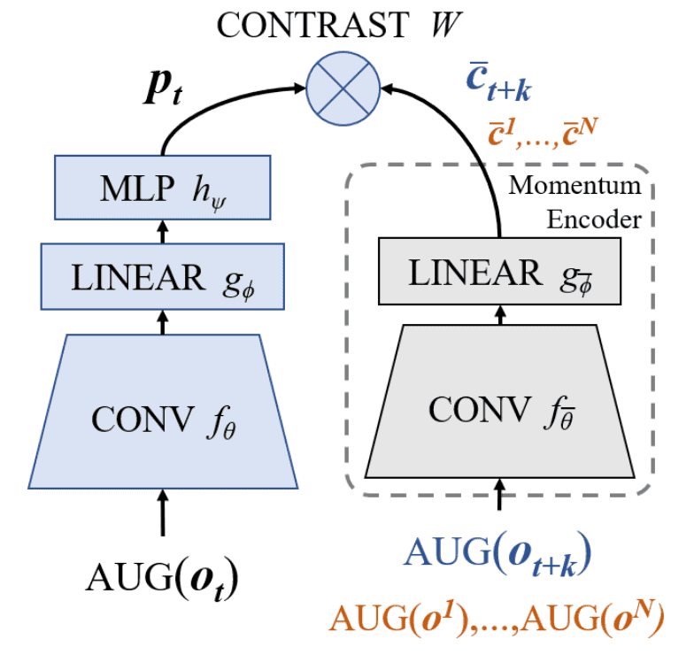
ATC requires a model to associate observations \(\mathbf{o}_t\) from nearby future timesteps \(\mathbf{o}_{t+k}\) within the same trajectory. ATC consists of four learned components:

1. Convolutional encoder $f_\theta$
   Observations $\mathbf{o}$ are encoded via a convolutional encoder $f_\theta$ (shared with the RL agent) into latent image $\mathbf{z}$: $$ \mathbf{z}_t = f_\theta ( \texttt{AUG} (\mathbf{o}_t) ) $$
2. Linear global compressor $g_\phi$
   A linear global compressor $g_\phi$ produces a small latent code vector $\mathbf{c}$: $$ \mathbf{c}_t = g_\phi (\mathbf{z}_t) $$ The contrastive loss is applied in this small latent space.
3. Residual predictor $h_\psi$
   A residual predictor $h_\psi$ advances the code $\mathbf{c}$ as an implicit forward model: $$ \mathbf{p}_t = h_\psi (\mathbf{c}_t) + \mathbf{c}_t $$
4. Contrastive transformation matrix $\mathbf{W}$
   A contrastive transformation matrix $\mathbf{W}$ is used to compute the bilinear similarity. In ATC, the positive observation $\mathbf{o}_{t+k}$ of an anchor $\mathbf{o}_t$ is processed into the target code: $$ \bar{\mathbf{c}}_{t+k} = g_\bar{\phi} (f_{\bar{\theta}} (\texttt{AUG} (\mathbf{o}_{t+k}))) $$ where the target encoder $f_{\bar{theta}}$ and global compressor $g_{\bar{\phi}}$ are EMA versions of online networks: $$ \begin{aligned} \bar{\theta} & \leftarrow (1 - \tau) \bar{\theta} + \tau \theta \\ \bar{\phi} & \leftarrow (1 - \tau) \bar{\phi} + \tau \phi \\ \end{aligned} $$ Then the contrastive loss is computed by InfoNCE loss: $$ \mathcal{L}_\texttt{ATC} = - \mathbb{E}_\mathcal{O} \left[ \log \frac{\exp \ell_{i, i+}}{\sum_{\mathbf{o}_j \in \mathcal{O}} \exp \ell_{i, j+} }\right] $$ where $\ell = \mathbf{p}_t \mathbf{W} \bar{\mathbf{c}}_{t + k}$ is the logit and $\mathbf{o}_{i+}$ are the positive observations of the given observation $\mathbf{o}_i \in \mathcal{O}$.

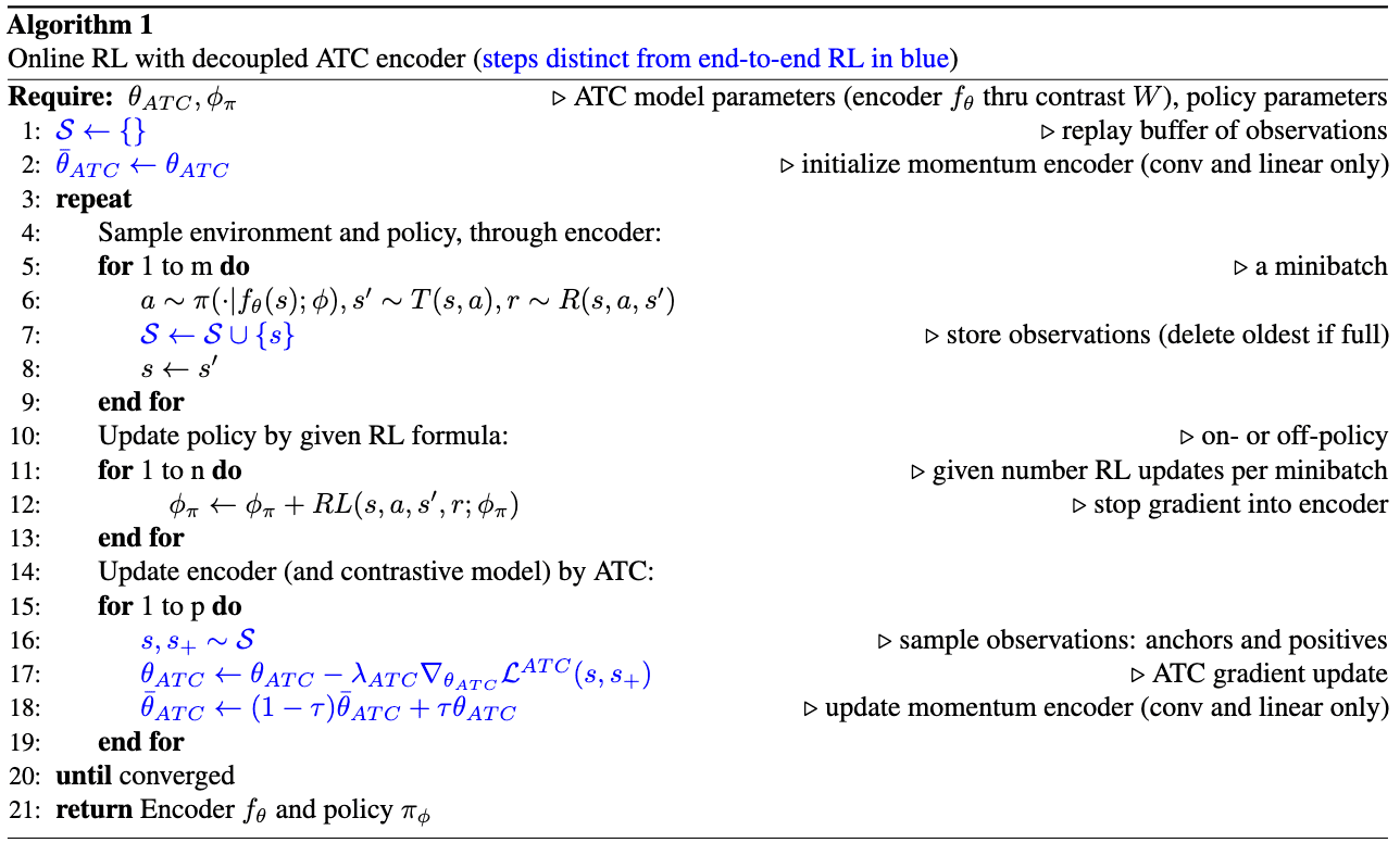
Note that these training steps do not necessitate RL reward as a learning signal. The following pseudocode shows the overall ATC algorithm in online RL framework.

$\mathbf{Fig\ 6.}$ ATC with online RL algorithm (Stooke et al. 2020)

Self-Predictive Representation Learning

Self-Predictive Representations (SPR)

Self-Predictive Representations (SPR), introduced by Schwarzer et al. ICLR 2021, enhances state representations for RL by employing a contrastive learning framework that compels representations to be temporally predictive and consistent when subjected to data augmentation.

$\mathbf{Fig\ 7.}$ SPR framework (Schwarzer et al. 2021)

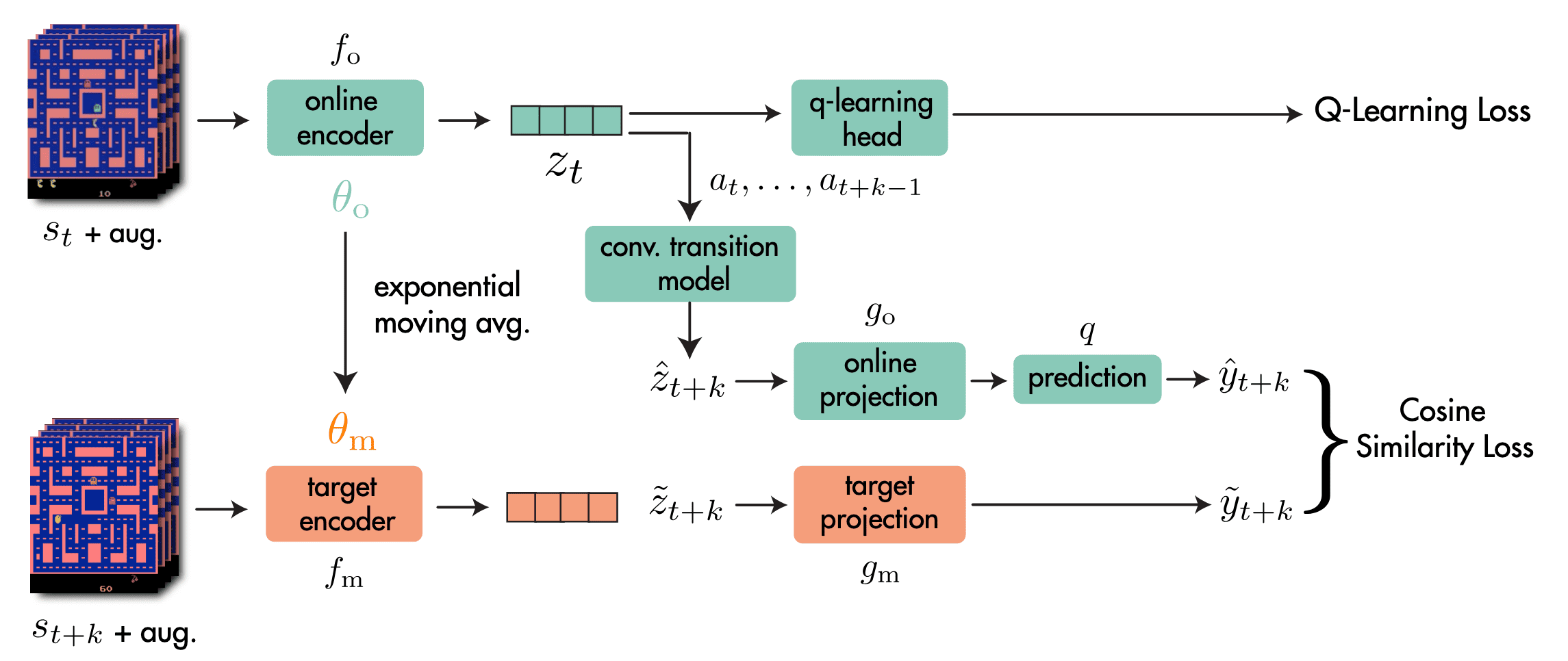
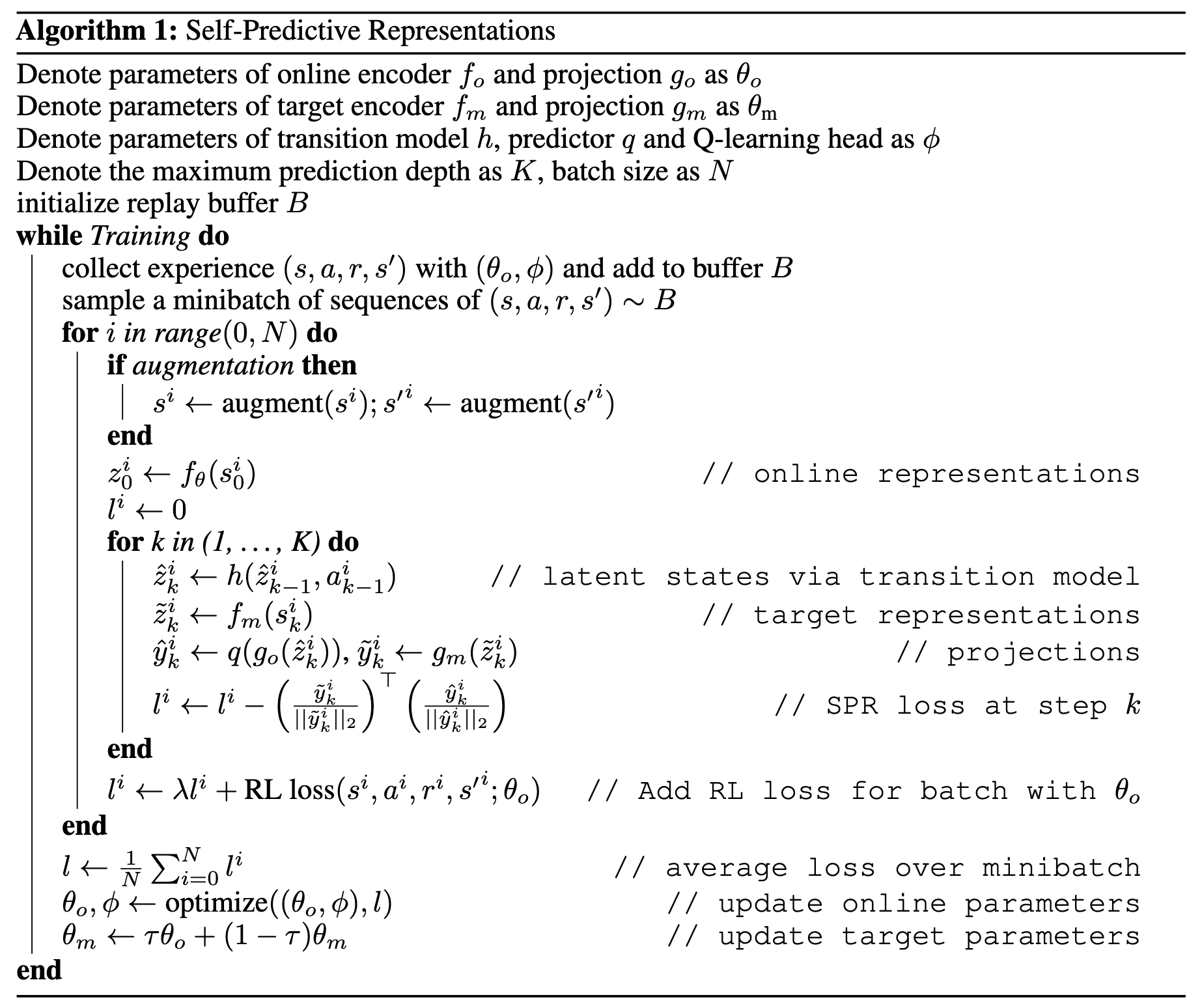
Let \((\mathbf{s}_{t:t+K}, \mathbf{a}_{t:t+K})\) denote a sequence of $K + 1$ previously experienced states and actions sampled from replay buffer $\mathcal{B}$ ($k = 5$ in practice). The SPR method consists of 4 main components:

1. Online & Target Networks $f_\mathrm{o}$, $f_\mathrm{m}$
   Analogous to popular self-supervised learning methods, the SPR framework has online network $f_\mathrm{o}$ and target network $f_\mathrm{m}$ to extract representations $\mathbf{z}_t$ from the observed states $\mathbf{s}_t$ with data augmentation. $$ \begin{aligned} \mathbf{z}_t & = f_\mathrm{o} (\mathbf{s}_t) \\ \tilde{\mathbf{z}}_t & = f_\mathrm{m} (\mathbf{s}_t) \end{aligned} $$ For each networks, each observation $\mathbf{s}_t$ independently augmented. Denoting the parameters of $f_\mathrm{o}$ as $\theta_\mathrm{o}$, those of $f_\mathrm{m}$ as $\theta_\mathrm{m}$, the update rule for $\theta_\mathrm{m}$ is EMA: $$ \theta_\mathrm{m} \leftarrow \tau \theta_\mathrm{m} + (1-\tau) \theta_\mathrm{o} $$ In practice, these encoders are implemented using he 3-layer convolutional encoder of DQN.
2. Transition Model $h$
   For the prediction objective, the SPR framework generates $K$ predictions $\mathbf{z}_{t+1:t+K}$ of future state representations $\tilde{\mathbf{z}}_{t+1:t+K}$ using an action-conditioned transition model $h$: $$ \begin{aligned} \mathbf{z}_{t+k+1} & = h (\mathbf{z}_{t+k}, \mathbf{a}_{t+k}) \\ \tilde{\mathbf{z}}_{t+k} & = f_\mathrm{m} (\mathbf{s}_{t+k}) \end{aligned} $$ starting from $\mathbf{z}_t = f_\mathrm{o} (\mathbf{s}_t)$.
3. Projection Heads $g_\mathrm{o}$, $g_\mathrm{m}$
   To avoid the loss of information in the representations extracted by encoders $f$, the projection heads $g_\mathrm{o}$ and $g_\mathrm{m}$ are attached that project online and target representations to a smaller latent space. Also, an additional prediction head $q$ to the online projections: $$ \begin{aligned} \mathbf{y}_{t+k} & = q (g_\mathrm{o} (\mathbf{z}_{t+k})) \\ \tilde{\mathbf{y}}_{t+k} & = g_\mathrm{m} (\tilde{\mathbf{z}}_{t+k}) \end{aligned} $$ The $g_\mathrm{m}$ parameters are also given by an EMA of the $g_\mathrm{o}$ parameters. In practice, the first layer of the DQN MLP head is reused as the SPR projection head.
4. Prediction Loss $\mathcal{L}_\theta^\texttt{SPR}$
   The future prediction loss for SPR is computed by summing over cosine similarities between the predicted and observed representations at timesteps $t + k$ for $1 \leq k \leq K$: $$ \mathcal{L}_\theta^\texttt{SPR} (\mathbf{s}_{t:t+K}, \mathbf{a}_{t:t+K}) = - \sum_{k=1}^K \left( \frac{\mathbf{y}_{t+k}}{\Vert \mathbf{y}_{t+k} \Vert_2 } \right)^\top \left( \frac{\tilde{\mathbf{y}}_{t+k}}{\Vert \tilde{\mathbf{y}}_{t+k} \Vert_2 } \right) $$ During training, the SPR loss is combined with the RL loss as an auxiliary loss, yielding the following full optimization objective: $$ \mathcal{L}_\theta^\texttt{total} = \mathcal{L}_\theta^\texttt{RL} + \lambda \mathcal{L}_\theta^\texttt{SPR} $$ Here, the SPR loss affects $f_\mathrm{o}$, $g_\mathrm{o}$, $q$, and $h$ and the RL loss affects $f_\mathrm{o}$ and the additional head attached to the encoder for the RL algorithm (e.g., in Rainbow, Q-learning head to estimate the Q-value from $\mathbf{z}$). In practice, the calculation of the SPR loss at episode boundaries are truncated to avoid encoding environment reset dynamics into the model.

$\mathbf{Fig\ 8.}$ The pseudocode of SPR (Schwarzer et al. 2021)

Experimental Results

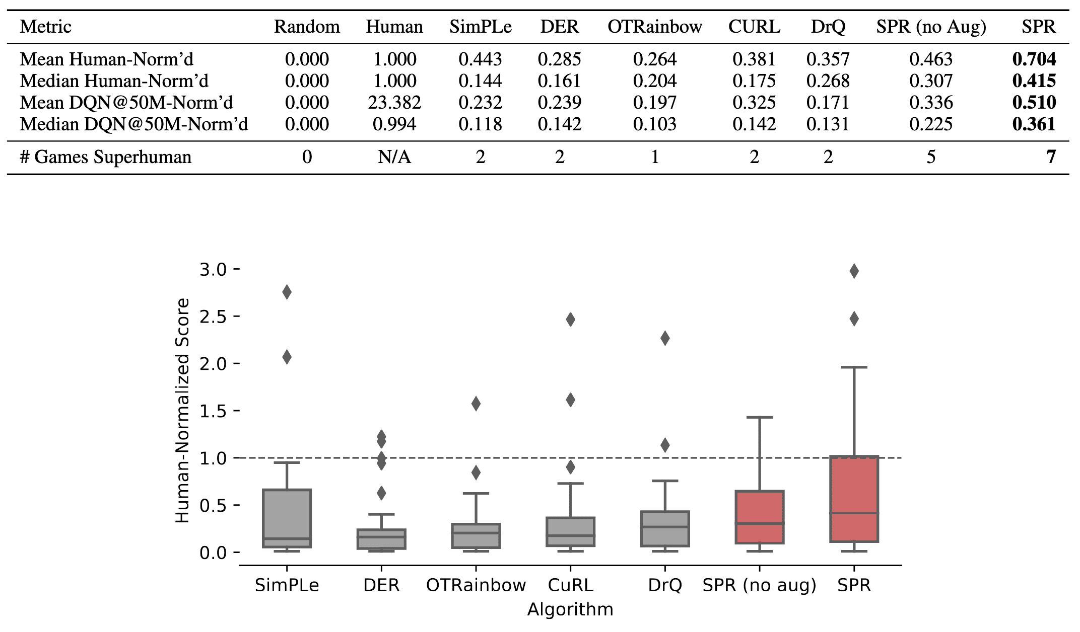
When combined with data augmentation, SPR attains a median human-normalized score of $0.415$, setting a state-of-the-art result fpr Atari-$100\mathrm{k}$ tasks. Also, SPR exhibits super-human performance on seven games within this data-limited setting: Boxing, Krull, Kangaroo, Road Runner, James Bond and Crazy Climber, surpassing the maximum of two achieved by any prior methods.

$\mathbf{Fig\ 9.}$ Performance of different methods on the Atari after $100\mathrm{k}$ environment steps (Schwarzer et al. 2021)

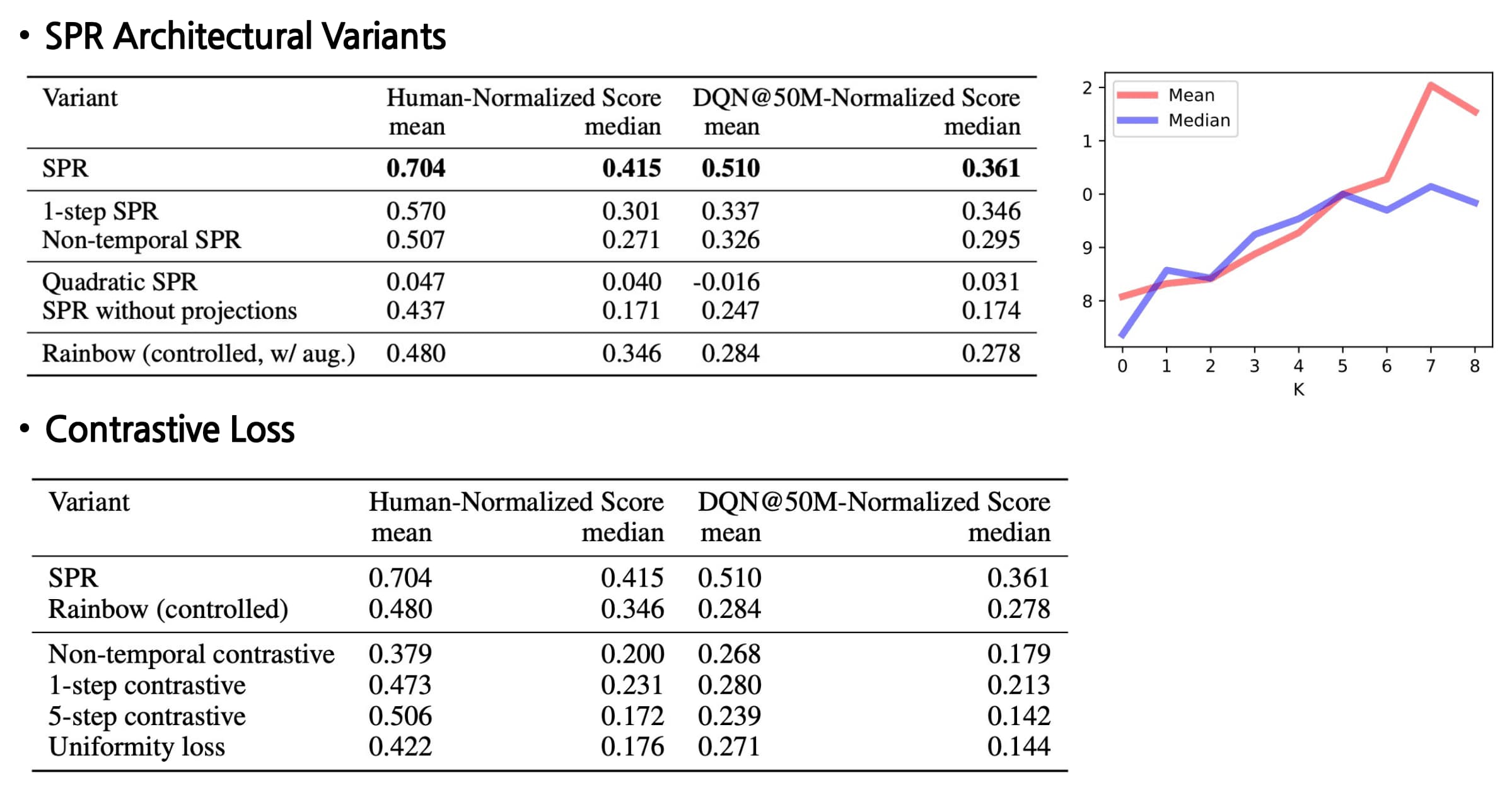
In addition, the ablations on SPR method provides several insights:

• Dynamics modeling is key
  A key distinction between SPR and other approaches is the incorporation of an explicit multi-step dynamics model. The authors demonstrate that extended dynamics modeling consistently enhances performance up to approximately $K=5$.
• Comparison with contrastive losses
  Although many recent works in representation learning utilize contrastive learning, the authors found that SPR consistently outperforms both temporal and non-temporal variants of contrastive losses. Additionally, employing a quadratic loss leads to representation collapse.
• Projections are critical
  SPR without projection and prediction heads has inferior performance, potentially because the effects of SPR in enforcing invariance to augmentation may be undesirable. The convolutional feature map, produced by only three layers, limits the ability to learn features that are both rich and invariant. Moreover, the convolutional network comprises only a small fraction of the capacity of SPR’s network, containing around 80,000 parameters out of a total of three to four million. By employing the first layer of the DQN head as a projection, the SPR objective can influence a much larger portion of the network, whereas its impact is restricted in this variant.

$\mathbf{Fig\ 10.}$ Ablation Studies on SPR (Schwarzer et al. 2021)

State & Action Representation Learning

Temporal Latent Action-Driven Contrastive Loss (TACO)

Previous works in visual RL has utilized additional self-supervised auxiliary tasks to enrich the agent’s representations with control-relevant information for predicting future states. However, these objectives often fall short of producing representations that fully capture the optimal policy or value function. This is because the positive relations in their contrastive losses are often policy-dependent, which can introduce instability during policy updates throughout training. Consequently, these methods lack a theoretical foundation robust enough to encapsulate all the information necessary to represent the optimal policy.

Zheng et al. NeurIPS 2023 learning an action representation that clusters semantically similar actions in latent action space can enable the agent to generalize its knowledge more effectively across diverse state-action pairs, enhancing the sample efficiency of RL algorithms. To achieve this, they introduced temporal latent action-driven contrastive loss (TACO) that learns both state and action representations for continuous control tasks.

$\mathbf{Fig\ 11.}$ Temporal contrastive loss of TACO (Zheng et al. 2023)

Let \(\mathbf{s}_t\) and \(\mathbf{a}_t\) be the states and actions at timestep $t$, \(\mathbf{z}_t = f_\phi (\mathbf{s}_t)\) and \(\mathbf{u}_t = f_\psi (\mathbf{a}_t)\) be their corresponding representations. TACO aims to maximize the mutual information $\mathcal{I}$ between representations of current states paired with action sequences and representations of the corresponding future states:

\[\begin{gathered} \mathcal{L}_\texttt{TACO} = \mathcal{I} (\mathbf{z}_{t+k}; \left[ \mathbf{z}_t, \mathbf{u}_t, \cdots, \mathbf{u}_{t+k-1} \right]) \\ \text{ where } \mathcal{I} (X; Y) = \mathrm{KL} (p (x, y) \Vert p(x) p(y)) = \mathbb{E}_{(X, Y) \sim p(x, y)} \left[ \log \frac{p(X, Y)}{p(X) p(Y)} \right] \end{gathered}\]

where $k$ is a fixed hyperparameter for the prediction horizon. By optimizing the mutual information between state and action representations, which measures the independence of them, TACO can be theoretically shown to capture the essential information to represent the optimal value function:

$\color{red}{\mathbf{Theorem.}}$ Sufficiency of $\mathcal{L}_\texttt{TACO}$
If for a given state and action representation $f_\phi$, $f_\psi$ and $\mathcal{L}_\texttt{TACO}$ is maximized, then for any state-action pairs $(\mathbf{s}_1, \mathbf{a}_1)$ and $(\mathbf{s}_2, \mathbf{a}_2)$ such that $f_\phi (\mathbf{s}_1) = f_\phi (\mathbf{s}_2)$ and $f_\psi (\mathbf{a}_1) = f_\psi (\mathbf{a}_2)$, it holds that $$ Q^* (\mathbf{s}_1, \mathbf{a}_1) = Q^* (\mathbf{s}_2, \mathbf{a}_2) $$

$\mathbf{Proof.}$

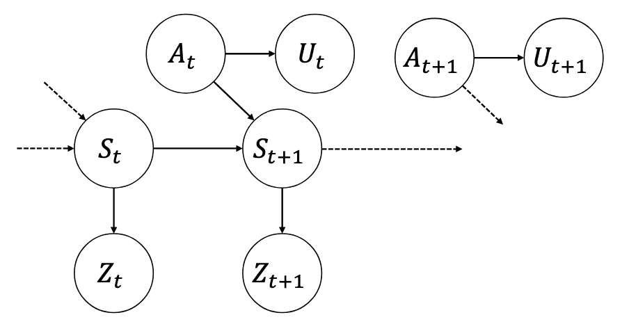
For the proof, consider the following graphical independence diagram:

The graphical diagram

We need two propositions to prove the main theorem:

$\color{#bf1100}{\mathbf{Proposition.}}$ Let $X$ be the return-to-go $\sum_{i=0}^{H - k - t} \gamma^i R_{t + k + i}$ with the conditional independence assumptions implied by the above graphical model. If $\mathcal{I}(Z_{t+k} ; Z_t, U_{t:t+k−1}) = \mathcal{I}(S_{t+K} ; S_t, A_{t:t+k-1})$, then $$ \mathcal{I}(X; Z_t, U_{t:t+k−1}) = \mathcal{I}(X; S_t, A_{t:t+k−1}) $$

$\mathbf{Proof.}$

We prove by contradictions. Suppose there exists a pair of state action representation $Z$, $U$, and a reward function $r$ such that $\mathcal{I}(Z_{t+k} ; Z_t, U_{t:t+k−1}) = \mathcal{I}(S_{t+k} ; S_t, A_{t:t+k−1})$, but

\[\mathcal{I}(X; Z_t, U_{t:t+k−1}) < \mathcal{I}(X; S_t, U_{t:t+k−1}) < \mathcal{I}(X; S_t, A_{t:t+k−1})\]

Then, it suffices to show that $\mathcal{I}(S_{t+k} ; Z_t, U_{t:t+K-1}) < \mathcal{I}(S_{t+k}; S_t, U_{t:t+k-1})$ since it gives us the desired contradiction $\mathcal{I} (Z_{t+k}; Z_t, U_{t: t+k-1}) \leq \mathcal{I} (S_{t+k}; S_t, U_{t: t+k-1})$, and $\mathcal{I}(S_{t+k}; S_t, U_{t:t+k-1}) \leq \mathcal{I} (S_{t+k}; S_t, A_{t:t+k-1})$.

By applying chain rule of mutual information to $\mathcal{I} (X; Z_t, S_t, U_{t:t+k-1})$:

\[\begin{aligned} \mathcal{I} (X; Z_t, S_t, U_{t:t+k-1}) & = \mathcal{I} (X; Z_t \vert S_t, U_{t:t+k-1}) + \mathcal{I} (X; S_t, U_{t:t+k-1}) \\ & = 0 + \mathcal{I} (X; S_t, U_{t:t+k-1}) \end{aligned}\]

Applying the chain rule in another way, we obtain:

\[\mathcal{I} (X; Z_t, S_t, U_{t:t+k-1}) = \mathcal{I} (X; S_t \vert Z_t, U_{t:t+k-1}) + \mathcal{I} (X; Z_t U_{t:t+k-1})\]

since our assumption of inequality $\mathcal{I}(X; Z_t, U_{t:t+k−1}) < \mathcal{I}(X; S_t, U_{t:t+k−1})$ and the mutual information must be $\geq 0$. Therefore:

\[\mathcal{I} (X; S_t, U_{t:t+k-1}) = \mathcal{I} (X; S_t \vert Z_t, U_{t:t+k-1}) + \mathcal{I} (X; Z_t, U_{t:t+k-1})\]

By our assumption that $\mathcal{I} (X; Z_t, U_{t:t+k-1}) < \mathcal{I} (X; S_t, U_{t:t+k-1})$, we must have:

\[\mathcal{I} (X; S_t \vert Z_t, U_{t:t+k-1}) > 0\]

Next, we expand $\mathcal{I} (S_{t+k}; Z_t, S_t, U_{t:t+k-1})$:

\[\begin{aligned} \mathcal{I} (S_{t+k}; Z_t, S_t, U_{t:t+k-1}) & = \mathcal{I} (S_{t+k}; Z_t \vert S_t, U_{t:t+k-1}) + \mathcal{I} (S_{t+k} ; S_t, U_{t:t+k-1}) \\ & = 0 + \mathcal{I} (S_{t+k} ; S_t, U_{t:t+k-1}) \end{aligned}\]

Therefore:

\[\mathcal{I} (S_{t+k}; S_t \vert Z_t, U_{t:t+k-1}) + \mathcal{I} (S_{t+k}; Z_t, U_{t:t+k-1}) = \mathcal{I} (S_{t+k}; Z_t, U_{t:t+k-1})\]

But then because $\mathcal{I}(S_{t+k}; S_t \vert Z_t, U_{t:t+k−1}) > \mathcal{I}(X; S_t \vert Z_t, U_{t:t+k−1})$ as $S_t \to S_{t+K} \to X$ forms a Markov chain, it is greater than zero by the inequality $\mathcal{I} (X; S_t \vert Z_t, U_{t:t+k-1}) > 0$. As a result:

\[\mathcal{I}(S_{t+K}; Z_t, U_{t:t+k−1}) < \mathcal{I}(S_{t+K}; S_t, U_{t:t+k−1}) < \mathcal{I}(S_{t+K}; S_t, A_{t:t+k−1}).\] \[\tag*{$\blacksquare$}\]

$\color{#bf1100}{\mathbf{Proposition.}}$ Let $X$, $Y$, $Z$ be random variables. Suppose $\mathcal{I} (Y, Z) = \mathcal{I} (Y, X)$ and $Y \perp Z \vert X$. THen, there exists a distribution $p(Z \vert X)$ such that: $$ p (Y \vert X = x) = \int p (Y \vert Z) p (Z \vert X = x) \; \mathrm{d}z $$ for any $x$.

$\mathbf{Proof.}$

Another way to write what we want to show is:

\[\mathrm{KL} \left[ p (Y \vert X) \Vert \mathbb{E}_{p(Z \vert X)} [p (Y \vert Z)] \right] = 0\]

The strategy of proof is to upper-bound this KL by a quantity that we will show to be $0$. Since KL divergences are always lower-bounded by $0$, this will prove equality. We begin by writing out the definition of the KL divergence, and then using Jensen’s inequality to upper-bound it:

\[\begin{aligned} \mathrm{KL} \left[ p (Y \vert X) \Vert \mathbb{E}_{p(Z \vert X)} [p (Y \vert Z)] \right] & = \mathbb{E}_{p (Y \vert X)} \log \left[ \frac{p(Y \vert X)}{\mathbb{E}_{p(Z \vert X)} [p (Y \vert Z)]} \right] \\ & = \mathbb{E}_{p (Y \vert X)} \left[ \log p(Y \vert X) - \log \mathbb{E}_{p(Z \vert X)} [p (Y \vert Z)] \right] \\ & \leq \mathbb{E}_{p (Y \vert X)} \left[ \log p(Y \vert X) - \mathbb{E}_{p(Z \vert X)} [\log p (Y \vert Z)] \right] \end{aligned}\]

Since KL divergences are greater than $0$, this last expression is also greater than $0$. Now let us try to relate $\mathcal{I}(Y; Z) = \mathcal{I}(Y ; X)$ to this expression. We can re-write this equality using the entropy definition of mutual information $\mathcal{I} (X; Y) = \mathbb{H} (X) - \mathbb{H} (X \vert Y)$:

\[\mathbb{H} (Y) - \mathbb{H} (Y \vert Z) = \mathbb{H} (Y) - \mathbb{H} (Y \vert X)\]

Therefore we have:

\[\mathbb{E}_{p(Y,Z)} \log p(Y \vert Z) = \mathbb{E}_{p(Y,X)} \log p(Y \vert X)\]

On the RHS, we can use the Tower property to re-write the expectation as:

\[\mathbb{E}_{p (Y, X)} \log p (Y \vert X) = \mathbb{E}_{p(Z)} \mathbb{E}_{p(Y, X \vert Z)} \log p(Y \vert X) = \mathbb{E}_{p (Y \vert X) p (X, Z)} \log p(Y \vert X)\]

Now we can use the Tower property again to re-write the expectation on both sides.

\[\begin{aligned} & \mathbb{E}_{p(X)} \mathbb{E}_{p(Y, Z \vert X)} \log p(Y \vert Z)=\mathbb{E}_{p(X)} \mathbb{E}_{p(Y \vert X) p(X, Z \vert X)} \log p(Y \vert X) \\ & \mathbb{E}_{p(X)} \mathbb{E}_{p(Y \vert X) p(Z \vert X)} \log p(Y \vert Z)=\mathbb{E}_{p(X)} \mathbb{E}_{p(Y \vert X) p(Z \vert X)} \log p(Y \vert X) \\ & \mathbb{E}_{p(X)} \mathbb{E}_{p(Y \vert X) p(Z \vert X)}[\log p(Y \vert X)-\log p(Y \vert Z)]=0 \\ & \mathbb{E}_{p(X)} \mathbb{E}_{p(Y \vert X)}\left[\log p(Y \vert X)-\mathbb{E}_{p(Z \vert X)} \log p(Y \vert Z)\right]=0 \end{aligned}\]

Because we know that $\mathbb{E}{p (Y \vert X)} \left[ \log p(Y \vert X) - \mathbb{E}{p(Z \vert X)} [\log p (Y \vert Z)] \right] \geq 0$ from the KL divergence inequality and the sum of elements that all have the same sign is zero, this implies each element is zero. Therefore:

\[0 = \mathbb{E}_{p (Y \vert X)} \left[ \log p(Y \vert X) - \mathbb{E}_{p(Z \vert X)} [\log p (Y \vert Z)] \right] \geq \mathrm{KL} \left[ p (Y \vert X) \Vert \mathbb{E}_{p(Z \vert X)} [p (Y \vert Z)] \right].\] \[\tag*{$\blacksquare$}\]

Based on the graphical model, it is clear that:

\[\max_{\phi, \psi} \mathcal{I} (Z_{t + k}, [Z_t, U_t, \cdots, U_{t+k-1}]) = \mathcal{I} (S_{t+k}, [S_t, A_t, \cdots, A_{t + k - 1}])\]

Now, define the random variable of return-to-go $\bar{R}_t$ such that:

\[\bar{R}_t = \sum_{k=0}^{H-t} \gamma^k R_{t+k}\]

Based on the first proposition, because

\[\mathcal{I} (Z_{t+k}; Z_t, U_{t:t+k-1}) = \mathcal{I} (S_{t+k}; S_t, A_{t:t+k-1})\]

we could conclude that

\[\mathcal{I} (\bar{R}_{t+k}; Z_t, U_{t+k-1}) = \mathcal{I} (\bar{R}_{t+k}; S_t, A_{t+k-1})\]

Now, applying the second proposition, we obtain:

\[\mathbb{E}_{p (\mathbf{z}_t, \mathbf{u}_{t:t+k-1} \vert S_t = \mathbf{s}, A_{t:t+k-1} = \mathbf{a}_{t:t+k-1})} [ p(\bar{R}_t \vert Z_t, U_{t:t+k-1}) ] = p(\bar{R}_t \vert S_t = \mathbf{s}, A_{t:t+k-1})\]

Consequently, when $k = 1$, or any reward function $r$, given a state-action pair \((\mathbf{s}_1, \mathbf{a}_1)\), \((\mathbf{s}_2, \mathbf{a}_2)\) such that \(f_\phi(\mathbf{s}_1) = f_\phi(\mathbf{s}_2)\), \(f_\psi(\mathbf{a}_1) = f_\psi(\mathbf{a}_2)\), we have \(Q_r (\mathbf{s}_1, \mathbf{a}_1) = \mathbb{E}_{p(R_t \vert S_t = \mathbf{s}_1, A_t = \mathbf{a}_1)}[\bar{R}_t] = \mathbb{E}_{p(R_t \vert S_t = \mathbf{s}_2, A_t = \mathbf{a}_2)}[\bar{R}_t] = Q_r (\mathbf{s}_2, \mathbf{a}_2)\). This is because \(p(\bar{R}_t \vert S_t = \mathbf{s}_1, A_t = \mathbf{a}_1) = p(\bar{R}_t \vert S_t = \mathbf{s}_2, A_t = \mathbf{a}_2)\) as \(p(\mathbf{z}_t \vert S_t = \mathbf{s}_1) = p(\mathbf{z}_t \vert S_t = \mathbf{s}_2)\), \(p(\mathbf{u}_t \vert A_t = \mathbf{a}_1) = p(\mathbf{u}_t \vert A_t = \mathbf{a}_2)\).

In case when $k > 1$, because if $\mathbb{E}[Z_{t+k} , [Z_t, U_t, \cdots, U_{t+k−1}]] = \mathbb{E}[S_{t+k}, [S_t, A_t, \cdots, A_{t+k−1}]]$, then for any $1 \leq i \leq k$, $\mathbb{E}[Z_{t+k}, [Z_t, U_t, \cdots, U_{t+i−1}]] = \mathbb{E}[S_{t+k}, [S_t, A_t, \cdots, A_{t+i−1}]]$, including $k = 1$, by Data processing Inequality. (Intuitively, this implies that if the information about the transition dynamics at a specific step is lost, the mutual information decreases as the timestep progresses, making it impossible to reach its maximum value at horizon $k$.) Then the same argument should also apply here.

\[\tag*{$\blacksquare$}\]

Note that the InfoNCE loss can be used as an alternative loss to maximize the mutual information. Given an instance $\mathbf{x} \sim p (\mathbf{x})$ and a corresponding positive sample $\mathbf{y}^+ \sim p(\mathbf{y} \vert \mathbf{x})$ and a colection of \(Y = \{ \mathbf{y}_1, \cdots, \mathbf{y}_{N-1} \}\) of $N -1$ random samples from $p(\mathbf{y})$, optimizing two losses are equivalent:

\[\begin{aligned} \mathcal{L}_{\texttt{InfoNCE}} & = - \mathbb{E}_\mathbf{x} \left[ \log \frac{f (\mathbf{x}, \mathbf{y}^+)}{ \sum_{\mathbf{y} \in Y \cup \{ \mathbf{y}^+ \}} f(\mathbf{x}, \mathbf{y})} \right] \\ & \geq - \mathbb{E}_\mathbf{x} \left[ \log \frac{p (\mathbf{y}^+ \vert \mathbf{x}) / p(\mathbf{y}^+)}{ \sum_{\mathbf{y} \in Y \cup \{ \mathbf{y}^+ \}} p (\mathbf{y} \vert \mathbf{x}) / p(\mathbf{y})} \right] \\ & = \mathbb{E}_\mathbf{x} \left[ \log \left( 1 + \frac{p(\mathbf{y}^+)}{p(\mathbf{y}^+ \vert \mathbf{x})} \cdot \sum_{\mathbf{y} \in Y} \frac{p (\mathbf{y} \vert \mathbf{x})}{p(\mathbf{y})} \right) \right] \\ & \approx \mathbb{E}_\mathbf{x} \left[ \log \left(1 + \frac{p(\mathbf{y}^+)}{p(\mathbf{y}^+ \vert \mathbf{x})} \cdot (N - 1) \mathbb{E}_{\mathbf{y} \sim p(\mathbf{y})} \left[ \frac{p (\mathbf{y} \vert \mathbf{x})}{p(\mathbf{y})} \right] \right) \right] \text{ by MC approximation } \\ & = \mathbb{E}_\mathbf{x} \left[ \log \left(1 + \frac{p(\mathbf{y}^+)}{p(\mathbf{y}^+ \vert \mathbf{x})} \cdot (N - 1) \right) \right] \\ & \geq \mathbb{E}_\mathbf{x} \left[ \frac{p(\mathbf{y}^+)}{p(\mathbf{y}^+ \vert \mathbf{x})} \cdot N \right] = \log N - \mathcal{I} (X; Y^+) \end{aligned}\]

from the fact that the optimizer of the InfoNCE loss is $f(\mathbf{x}, \mathbf{y}) \propto \frac{p(\mathbf{y} \vert \mathbf{x})}{p(\mathbf{x})}$.

Practical Implementation of TACO loss

Based on the equivalence above, TACO estimates a lower bound of mutual information through the InfoNCE loss. In practical implementation, the authors found that adding two auxiliary objectives further boosts the algorithm’s overall performance. The complete TACO loss is therefore computed as a combination of following three losses with equal weight:

\[\mathcal{J}_\texttt{TACO} = \mathcal{L}_\texttt{TACO} + \mathcal{L}_\texttt{CURL} + \mathcal{L}_\texttt{Reward}\]

1. Temporal Latent Action-Driven Contrasitive Loss
   Given a batch of state-action transition triples $\{ (\mathbf{s}_t^{(i)}, [\mathbf{a}_t^{(i)}, \cdots, \mathbf{a}_{t+k-1}^{(i)}], \mathbf{s}_{t+k}^{(i)}) \}_{i=1}^N$, the state encoder and action encoder to get latent state-action encodings: $$ \mathbf{z}_t^{(i)} = f_\phi (\mathbf{s}_t^{(i)}), \quad \mathbf{u}_t^{(i)} = f_\psi (\mathbf{a}_t^{(i)}) $$ These latents are projected to the contrastive embedding space by two learnable projection $G_\theta, H_\theta$: $$ \mathbf{g}_t^{(i)} = G_\theta (\mathbf{z}_t^{(i)}, \mathbf{u}_t^{(i)}, \cdots, \mathbf{z}_{t + k - 1}^{(i)}), \quad \mathbf{h}_{t + k}^{(i)} = H_\theta (\mathbf{z}_{t + k}^{(i)}) $$ With learnable parameter $\mathbf{W}$ for bilinear similarity, the TACO loss is computed by InfoNCE loss: $$ \mathcal{L}_{\texttt{TACO}} (\phi, \psi, \mathbf{W}, G_\theta, H_\theta) = - \frac{1}{N} \sum_{i=1}^N \log \frac{ {\mathbf{g}_t^{(i)}}^\top \mathbf{W} \mathbf{h}_{t+k}^{(i)}}{\sum_{j=1}^N {\mathbf{g}_t^{(i)}}^\top \mathbf{W} \mathbf{h}_{t+k}^{(j)}} $$
2. CURL Loss
   Since the state encoding is one of the most challenging part in visual RL, the additional CURL loss of observations can improve the performance: $$ \mathcal{L}_\texttt{CURL} (\phi, \psi, \mathbf{W}, H_\theta) = - \frac{1}{N} \sum_{i=1}^N \log \frac{ {\mathbf{h}_t^{(i)}}^\top \mathbf{W} {\mathbf{h}_{t+k}^{(i)}}^+ }{ {\mathbf{h}_t^{(i)}}^\top \mathbf{W} {\mathbf{h}_{t+k}^{(i)}}^+ + \sum_{j \neq i}^N {\mathbf{h}_t^{(i)}}^\top \mathbf{W} \mathbf{h}_{t+k}^{(j)}} $$ where ${\mathbf{h}_t^{(i)}}^+ = H_\theta (f_\phi ({\mathbf{s}_t^{(i)}}^+))$ and ${\mathbf{s}_t^{(i)}}^+$ is the augmented view of $\mathbf{s}_t^{(i)}$. Here, $\mathbf{W}$ and $H_\theta$ share the same weight as the ones in $\mathcal{L}_\texttt{TACO}$.
3. Reward Prediction
   $$ \mathcal{L}_\texttt{reward} (\phi, \psi, \hat{R}_\theta) = \sum_{i=1}^N \left( \hat{R}_\theta ([\mathbf{z}_t^{(i)}, \mathbf{u}_t^{(i)}, \cdots, \mathbf{u}_{t + k - 1}^{(i)} ])- r^{(i)} \right)^2 $$ where $\hat{R}_\theta$ is a reward prediction head and $r^{(i)} = \sum_{j=t}^{t + k - 1} r_j^{(i)}$ is the sum of reward from timestep $t$ to $t + k - 1$.

In online RL setting, TACO is incorporated into the update function of existing visual RL algorithms as follows.

### Extract feature representation for state and actions.
def update(batch) :
  obs, action_sequence, reward, next_obs = batch
  ### Update Agent ’s critic function
  update_critic(obs, action_sequence, reward, next_obs)
  ### Update the agent ’s value function
  update_actor(obs)
  ### Update TACO loss
  update_taco(obs, action_sequence, reward, next_obs)

The following PyTorch-like pseudocode shows how TACO objective is implemented.

# state_encoder: State/Observation Encoder (CNN)
# action_encoder: Action Encoder (MLP with 1-hidden layer)
# sequence_encoder: Action Sequence encoder (Linear Layer)
# reward_predictor: Reward Prediction Layer (MLP with 1-hidden layer)
# G: Projection Layer I (MLP with 1-hidden layer)
# H: Projection Layer II (MLP with 1-hidden layer)
# aug: Data Augmentation Function (Radnom Shift)
# W: Matrix for computing similarity score
def compute_taco_objective (obs, action_sequence, reward, next_obs) :
  ### Compute feature representation for both state and actions.
  Z = state_encoder(aug(obs))
  z_anchor = state_encoder(aug(obs), stop_grad=True)
  next_z = state_encoder(aug(next_obs), stop_grad=True)
  u_seq = sequence_encoder(action_encoder(action_sequence))
  
  ### Project to joint contrastive embedding space
  x = G(torch.cat([z, u_seq], dim= 1))
  y = H(next_z)
  ### Compute bilinear product x^TWy
  logits = torch.matmul(x, torch.matmul (W, y.T))
  ### Diagonal entries of x^TWy correspond to positive pairs
  logits = logits - torch.max(logits, 1)
  labels = torch.arange(n)
  taco_loss = cross_entropy-loss (logits, labels)

  ### Compute CURL loss
  x = H(z)
  y = H(z_anchor).detach()
  logits = torch.matmul(x, torch.matmul (W, y.T))
  logits = logits - torch. max(logits, 1)
  labels = torch.arange(n)
  curl_loss = cross_entropy_loss(logits, labels)
  
  ### Reward Prediction Loss
  reward_pred = reward_predictor(z, u_seq)
  reward_loss = torch.mse_loss(reward_pred, reward)

  ### Entire Loss
  return taco-loss + curl_loss + reward_loss

Experimental Results

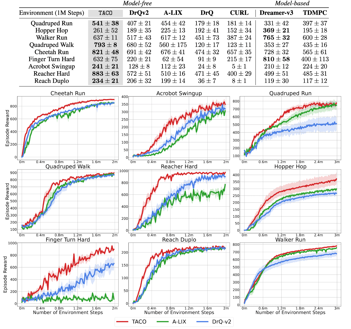
On vision-based Deepmind Control Suite and Meta-world benchmarks, TACO achieves a significantly better sample efficiency and performance compared with SOTA visual RL algorithm.

$\mathbf{Fig\ 12.}$ Comparisons on Vision-based Deepmind Control Suite (Zheng et al. 2023)

The authors demonstrated that jointly learning state and action representations is essential for TACO’s performance. Furthermore, the action representation successfully extracts control-relevant information from the raw action space.

In Cheetah Run task, they artificially introduced $20$ Gaussian-noised dimensions to the action space, although only the first $6$ were utilized in environmental interactions. The t-SNE results show that the TACO’s learned action representation effectively disregards these “noisy” dimensions while preserving information, forming four distinct clusters.

$\mathbf{Fig\ 13.}$ Effectiveness of action representation learning (Zheng et al. 2023)

Additionally, the following performance analysis of TACO loss indicates that:

1. The effectiveness of the temporal contrastive loss scales with increasing batch size.
2. Reward prediction and CURL losses act as auxiliary components to enhance TACO’s performance, while TACO’s temporal contrastive loss remains the most critical factor.

$\mathbf{Fig\ 14.}$ Performance analysis of TACO loss (Zheng et al. 2023)

References

[1] Laskin et al. “CURL: Contrastive Unsupervised Representations for Reinforcement Learning”, ICML 2020
[2] Stooke et al. “Decoupling Representation Learning from Reinforcement Learning”, PMLR 2021
[3] Zheng et al. “TACO: Temporal Latent Action-Driven Contrastive Loss for Visual Reinforcement Learning”, NeurIPS 2023
[4] Schwarzer et al., “Data-Efficient Reinforcement Learning with Self-Predictive Representations”, ICLR 2021