[RL] Enhancing Sample Efficiency in Visual RL

Training reinforcement learning (RL) agents directly from high-dimensional visual inputs is notoriously data-hungry. Learning from raw pixels often demands far more interactions than humans would need for the same tasks (Kaiser et al., ICLR 2020)​. This low sample efficiency–-the ability to learn effectively from limited experience–is a central challenge in deploying visual RL in the real world​. As a result, recent research must combine different domain-specific practices and auxiliary losses to learn meaningful behaviors in complex environments.

Regularization Methods

A-LIX of Cetin et al. ICML 2022 have introduced an adaptive regularization to convolutional features to mitigate catastrophic self-overfitting.

Adaptive Local Signal Mixing (A-LIX)

Cetin et al. 2022 provided an empirical evidence why applying successful off-policy RL algorithms designed for proprioceptive tasks to pixel-based environments is generally underwhelming. They claimed that three key elements strongly correlate with the occurrence of detrimental instabilities:

(i) Learning the critic’s weights solely from a TD learning objective
(ii) End-to-end backpropagation through unregularized CNN encoders
(iii) Low-magnitude, sparse environment rewards

which forms a new visual deadly triad.

$\mathbf{Fig\ 1.}$ Visual Deadly Triad (Cetin et al. 2022)

Visual Deadly Triad

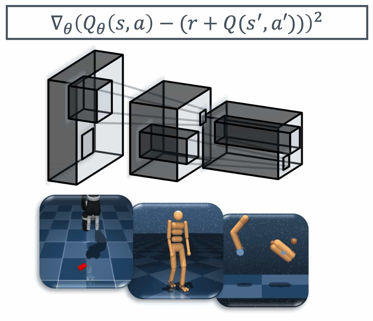
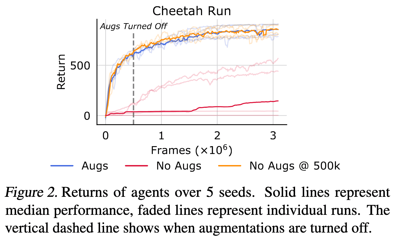
Unlike proprioceptive observations, off-policy RL from pixel observations commonly requires additional domain-specific practices, such as random shift augmentations, to ensure learning stability. Interestingly, the authors observed that augmentations are not needed for asymptotic performance, and are most helpful to counteract instabilities present in the earlier stages of learning.

$\mathbf{Fig\ 2.}$ Data Augmentations are most helpful at the earlier stages of training (Cetin et al. 2022)

To reduce confounding factors and to disentagle the origin of training instabilities, they designed a following experiment that isolates exploration, critic training, and actor training:

1. Using a random policy, gather a set of $15000$ transitions in vision-based Cheetah Run
2. Policy evaluation by training both critic and encoder using SARSA until convergence on this fixed data
3. Policy improvement by training an actor to maximize the expected discounted return as predicted by the converged critic

Interestingly,

• Turning on augmentations exclusively during exploration or policy improvement has no apparent effect on stability and final performance.
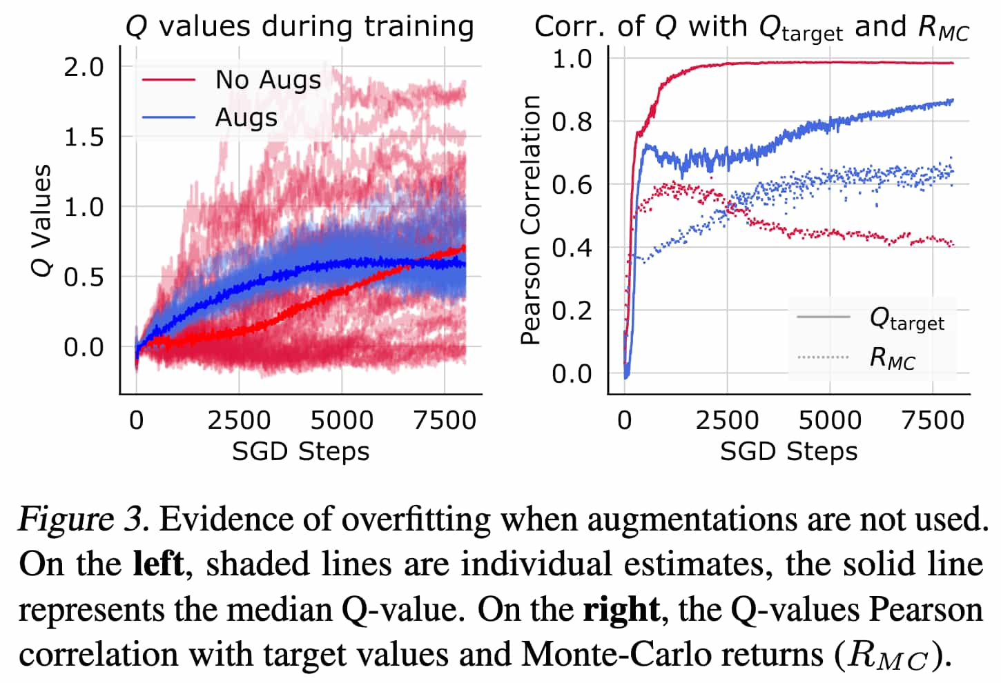
• When performing policy evaluation without augmentations, value predictions display extremely high variance across different state-action pairs.

$\mathbf{Fig\ 3.}$ Performance and training statistics of different agent types in the offline experiments from 15,000 random transitions (Cetin et al. 2022)

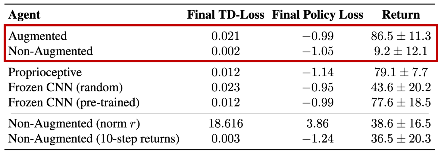
Note that the non-augmented critic exhibits a markedly lower loss, despite maintaining higher average Q-values than the augmented agent. This is an evident indication of overfitting. The progression of Pearson correlation between the estimated Q-values and both the target Q-values ($Q_\texttt{target}$) and the actual discounted Monte Carlo returns ($R_\texttt{MC}$) reveals that the non-augmented critic promptly learns to fit its own noisy, randomly-initialized predictions. They teremd this convergence to erroneous and high-variance Q-value predictions as a catastrophic self-overfitting.

$\mathbf{Fig\ 4.}$ Evidence of Overfitting (Cetin et al. 2022)

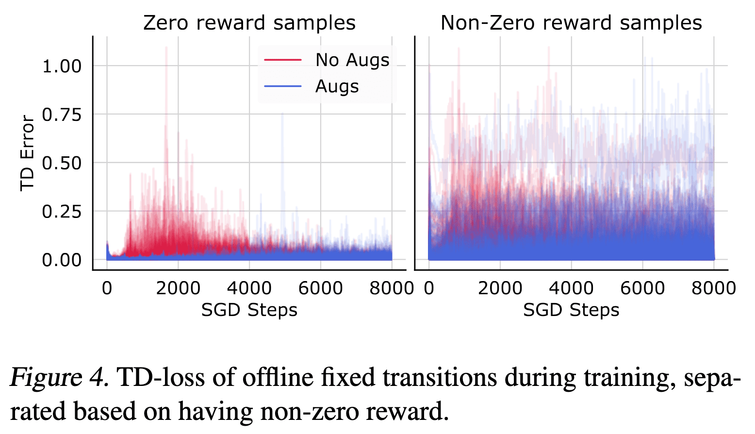
Hence, fitting the noisy targets severely affects learning the useful training signal from the collected transitions regarding the experienced rewards. This phenomenon is further confirmed by splitting the data into non-zero and zero reward transitions, where the only learning signal propagated in the TD-loss is from the initially random target values. As a result, the non-augmented agents initially experience much higher TD-errors on zero reward transitions, confirming that they focus on fitting uninformative components of the TD-objective.

$\mathbf{Fig\ 5.}$ Non-augmented agents focus on fitting uninformative components of the TD-objective (Cetin et al. 2022)

However, the authors caution that TD-learning is not the only cause for the observed instabilities.

1. Overfitting appears to be exclusive to performing end-to-end TD-learning with CNN encoders.
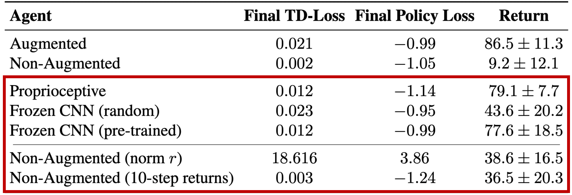
   When they trained a fully-connected critic network without training an encoder by considering three different (non-augmented image input, freezed to either randomly initialized weights or pre-trained from augmented agent) cases, they attain largely superior performance in all three cases.
2. Overfitting phenomenon is diminished when simply increasing the magnitude of the reward signal in the TD-loss
   Incorporating normalized reward and large $n$-step returns into critic learning considerably improve the non-augmented agent’s performance, although they still exhibit high variance.

$\mathbf{Fig\ 6.}$ Performance and training statistics of different agent types in the offline experiments from 15,000 random transitions (Cetin et al. 2022)

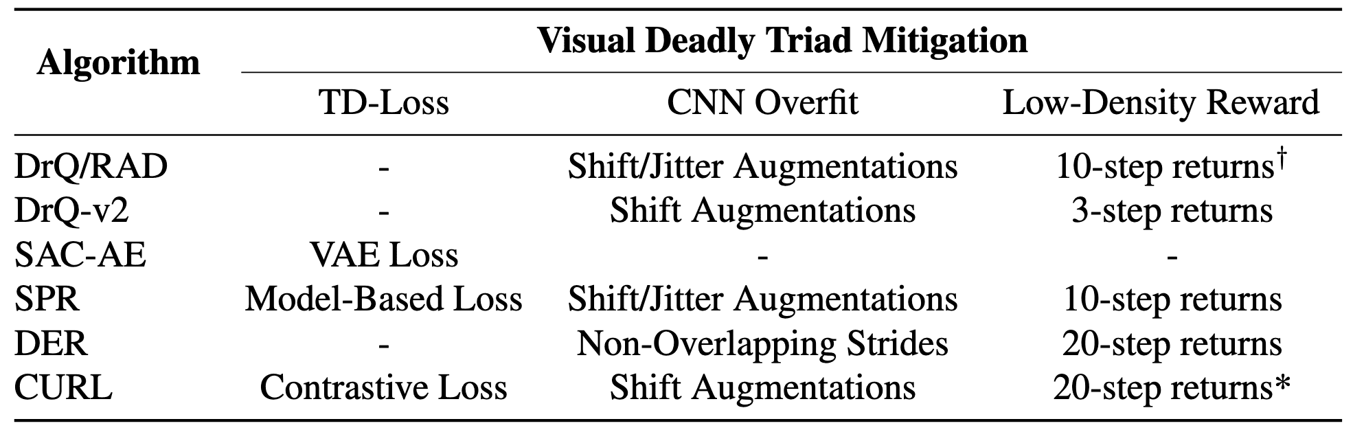
In summary, the authors argued that the training instabilities in vision-based reinforcement learning arise from three primary factors and termed visual deadly triad: (i) Exclusive reliance on the TD-loss; (ii) Unregularized learning with a highly expressive CNN encoder; (iii) initial low-magnitude sparse rewards. And they also contended that the successes of previous state-of-the-art visual RL algorithms are attributed to several domain-specific practices, summarized as follows:

$\mathbf{Fig\ 7.}$ Practices from recent pixel-based TD-learning methods to mitigate elements of the visual deadly triad (Cetin et al. 2022)

Catastrophic Self-Overfitting

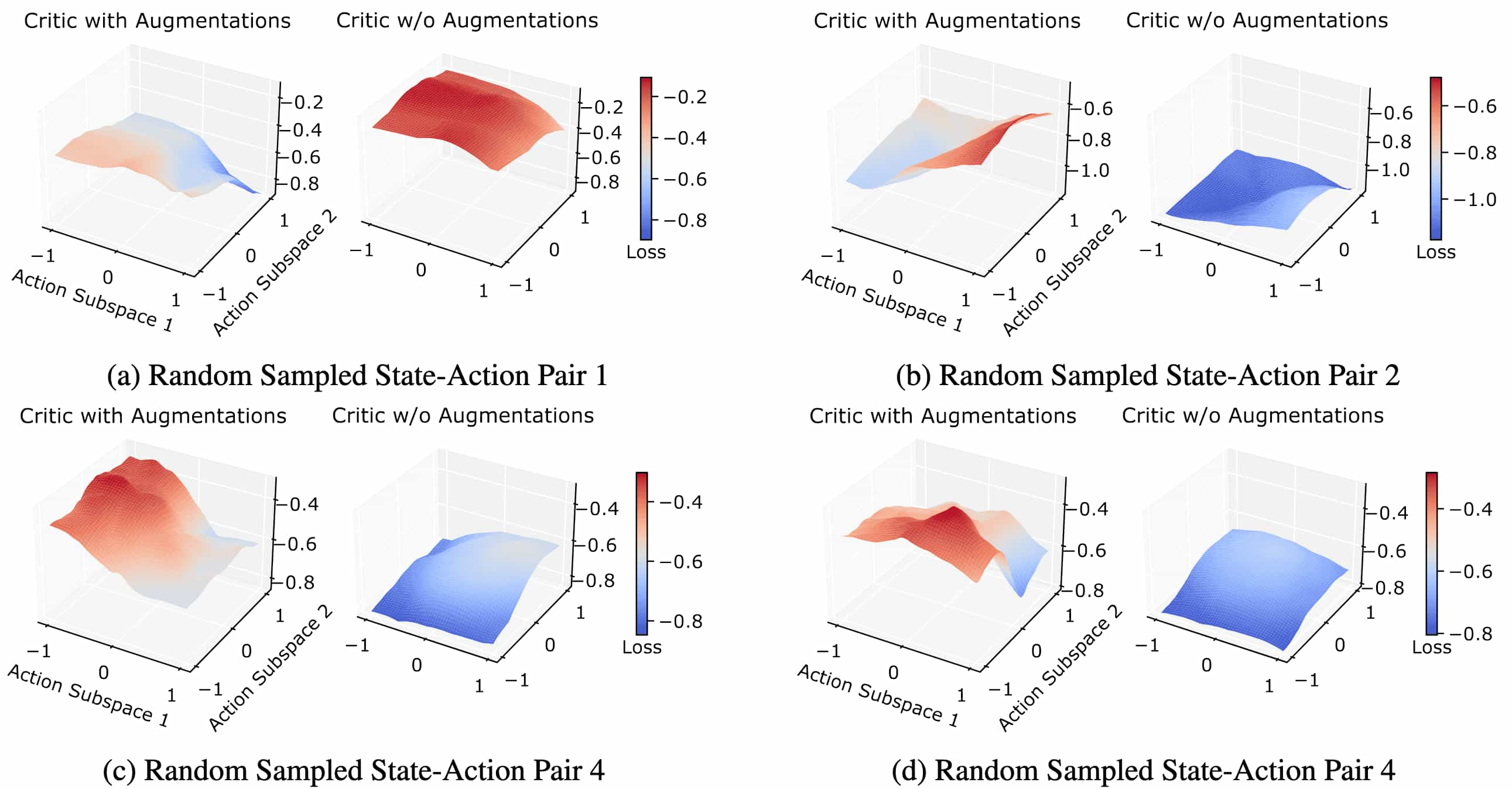
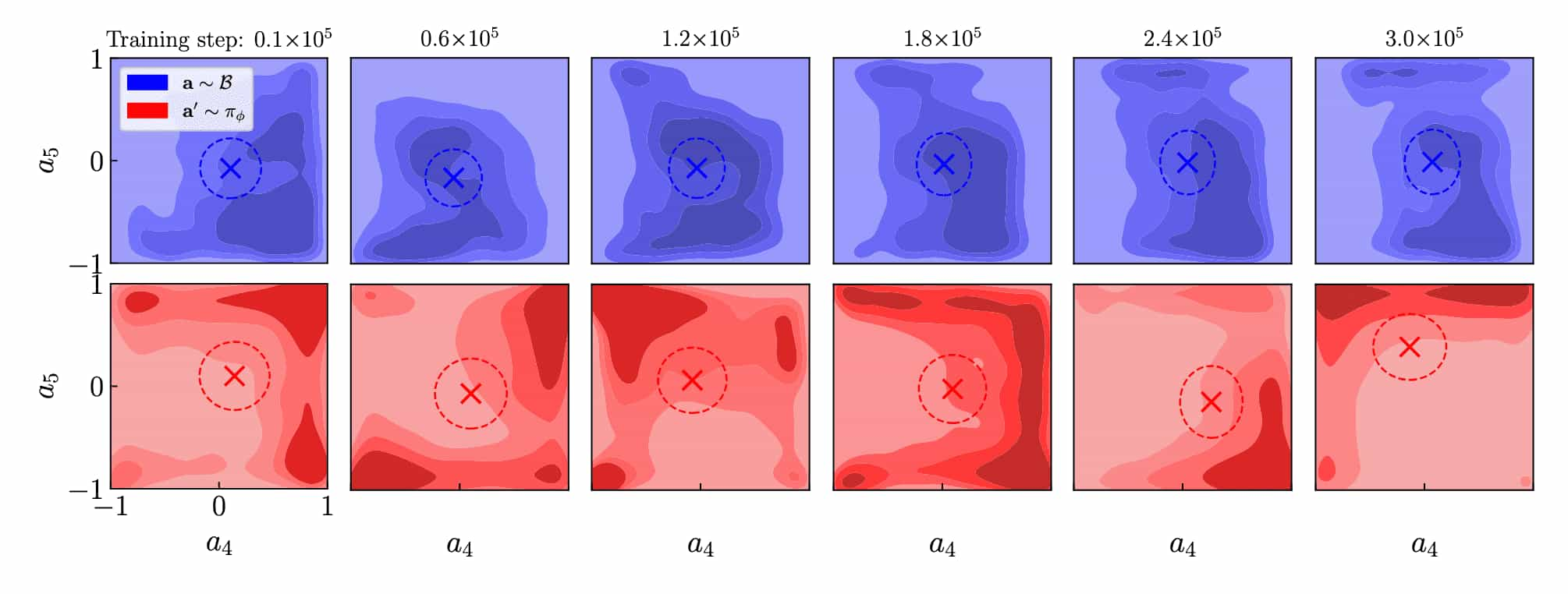
Specifically, the authors observed that catastrophic self-overfitting comes with a significant reduction of the critic’s sensitivity to changes in action inputs. See the following figure that illustrates the action-value surface plots. This implies that the erroneous high-variance Q-value predictions arise primarily due to changes in the observation.

$\mathbf{Fig\ 8.}$ Action-Value loss surface plotted with respect two orthogonal random directions sampled from the action space (Cetin et al. 2022)

To quantify the sensitivity of feature representations $\mathbf{z} \in \mathbb{R}^{C \times H \times W}$ to small perturbations $\boldsymbol{\epsilon}$ in the input observations $\mathbf{x}$, they computed the Frobenius norm of Jacobian of the encoder, measuring how quickly the encoder feature representations are changing locally around an input:

\[\Vert \mathbf{J} (\mathbf{x}) \Vert_F = \sum_{n} \sum_{m} \left( \frac{\partial \mathbf{F}_m (\mathbf{x})}{\partial \mathbf{x}_n} \right)^2 \text{ where } \mathbf{J} (\mathbf{x}) \approx \frac{\mathbf{F} (\mathbf{x} + \boldsymbol{\epsilon}) - \mathbf{F} (\mathbf{x})}{\boldsymbol{\epsilon}}\]

Consequently, the feature representations of the non-augmented agents being on average $2.85\times$ more sensitive, implying that overfitting is driven by the CNN encoder’s representations learning high-frequency information about the input observations and, thus, breaking useful inductive biases of CNN. The actual feature maps of different observation also shows that the feature map of non-augmented encoder has higher frequency with discontinuities, compared to an augmented one:

$\mathbf{Fig\ 9.}$ Feature maps in the final layer of encoder (Cetin et al. 2022)

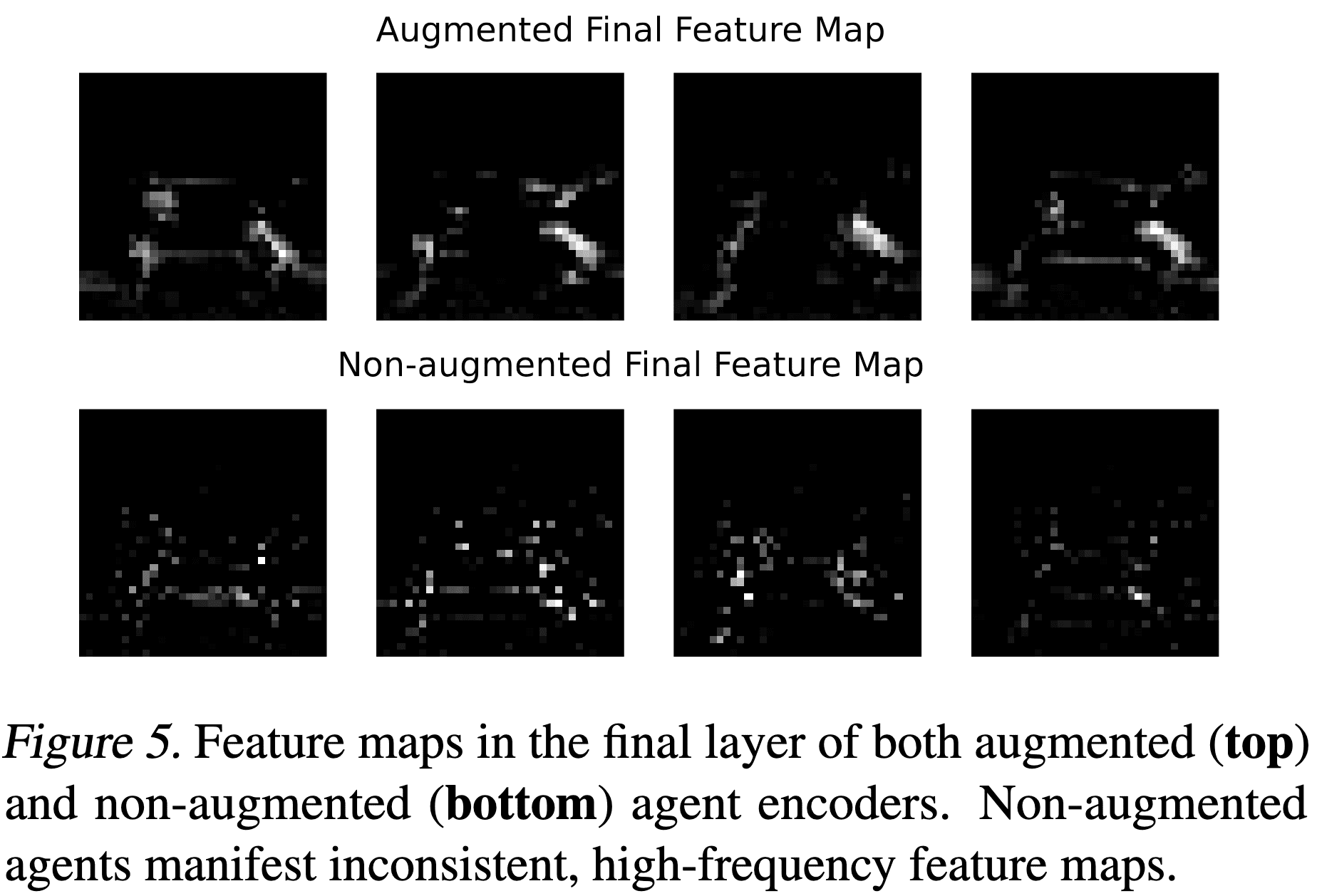
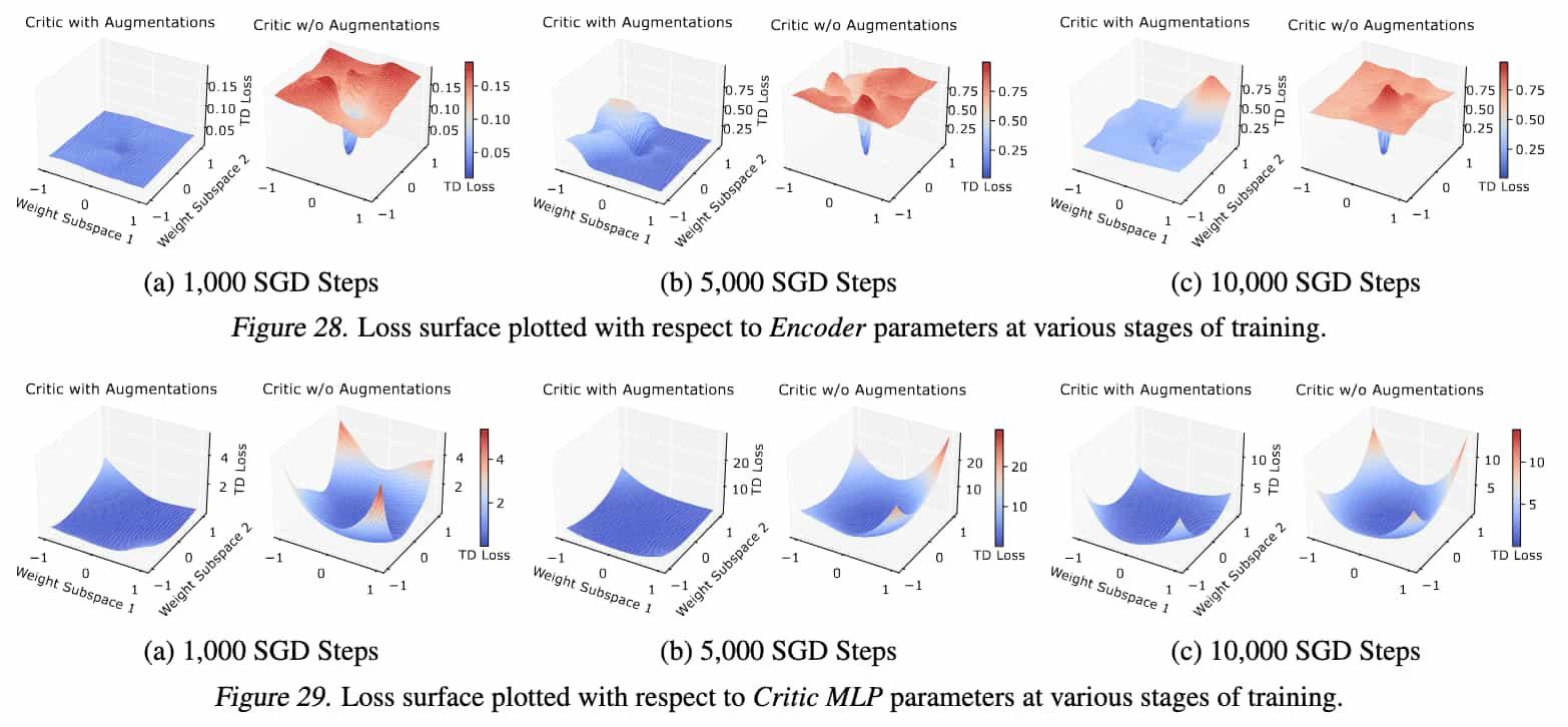
And importantly, the same phenomenon is also observed in the gradient of encoder’s parameters. Specifically, the gradients of the feature maps appear spatially consistent for the augmented agent, and discontinuous for the non-augmented agent. And we can conjecture that this impersistent discontinuous gradients should push the encoder’s weights to encode discontinuous representations.

Note that the loss surface with respect to the MLP parameters is significantly less sharp. Namely, it lends further evidence that self-overfitting is predominately a result of the flexibility of the CNN layers to learn high-frequency features.

$\mathbf{Fig\ 10.}$ Critic loss surface plots of augmented and non-augmented agent (Cetin et al. 2022)

Random shift provides implicit smoothing effect over the gradient maps

From the approximate shift invariance of convolutional layers, we can view a convolutional encoder as computing each of the feature vectors \([\mathbf{z}_{1ij} , \cdots, \mathbf{z}_{Cij} ]^\top\) with the same parameterized function $V_\phi$ (determined by kernel sizes, strides, …), that takes as input a subset of each observation \(\mathbf{o} \in \mathbb{R}^{C^\prime \times H^\prime \times W^\prime}\), which corresponds to a local neighborhood around some reference input coordinates \(i^\prime\), \(j^\prime\):

\[\mathbf{z}_{ij} = V_\phi (\mathcal{O}, i^\prime, j^\prime)\]

where some implicit function $f(i, j) = i^\prime, j^\prime$, determined by kernel sizes, strides, etc., translates each of the output features coordinate into the relative reference input coordinate. Random shifts are approximately equivalent to further translating each reference coordinate by adding some uniform random variables $\delta^\prime$:

\[\begin{gathered} \mathbf{z}_{ij} \approx V_\phi (\mathcal{O}, i^\prime + \delta_x^\prime, j^\prime + \delta_y^\prime) \\ \text{ where } \delta_x^\prime, \delta_y^\prime \sim \mathcal{U} [- s^\prime, s^\prime] \end{gathered}\]

Consequently, shift augmentations effectively turn the deterministic computation graph of each feature \(\mathbf{z}_{ij}\) into a random variable, whose sample space comprises the computation graphs of all nearby features within its feature map. Hence, applying different random shifts to samples in a minibatch makes the gradient \(\nabla \mathbf{z}_{ij}\) backpropagate to a random computation graph, and aggregating the parameter gradients produced with different $\delta$ provides a smoothing effect on the gradients and prevents persistent discontinuities.

Adaptive Local Signal Mixing

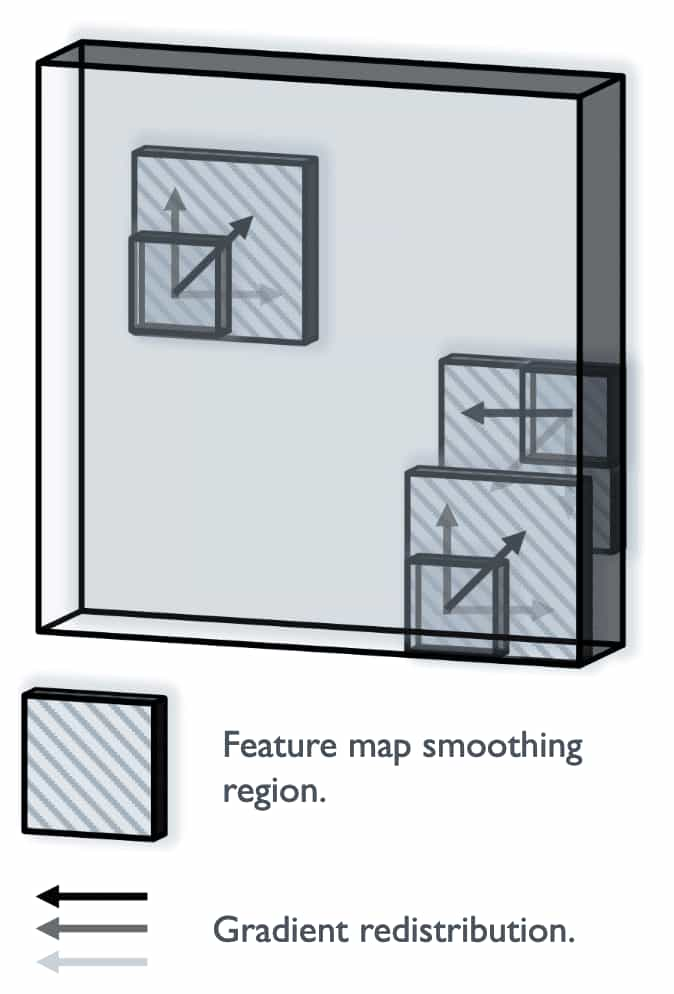
Inspired by the implicit regularization of random shift augmentation, Adaptive Local Signal Mixing (A-LIX) is a new neural network layer that aims to enforce gradient smoothing regularization explicitly to prevent catastrophic self-overfitting. It performs the weighted averaging as a bilinear interpolation with weights determined by the random shifts:

\[\begin{aligned} & \hat{\mathbf{z}}_{c i j}=\mathbf{z}_{c\lfloor\tilde{i}\rfloor\lfloor\tilde{j}\rfloor}(\lceil\tilde{i}\rceil-\tilde{i})(\lceil\tilde{j}\rceil-\tilde{j})+\mathbf{z}_{c\lfloor\tilde{i}\rfloor\lceil\tilde{j}\rceil} (\lceil\tilde{i}\rceil-\tilde{i})(\tilde{j}-\lfloor\tilde{j}\rfloor) \\ & +\mathbf{z}_{c\lceil \tilde{i} \rceil\lfloor \tilde{j} \rfloor}(\tilde{i}-\lfloor\tilde{i}\rfloor)(\lceil \tilde{j}\rceil-\tilde{j})+\mathbf{z}_{c\lceil \tilde{i} \rceil\lceil\tilde{j}\rceil}(\tilde{i}-\lfloor\tilde{i}\rfloor)(\tilde{j}-\lfloor\tilde{j}\rfloor). \end{aligned}\]

where $\tilde{i} = i + \delta_x$, $\tilde{j} = j + \delta_y$, and $\delta \sim \mathcal{U} (-s, s)$. Therefore, back propagation will split each gradient \(\nabla \hat{\mathbf{z}}_{c i j}\) to a random combination of features within the same feature map \(\{ \nabla \hat{\mathbf{z}}_{c \lfloor\tilde{i}\rfloor\lfloor\tilde{j}\rfloor}, \nabla \hat{\mathbf{z}}_{c \lfloor\tilde{i}\rfloor\lceil\tilde{j}\rceil}, \nabla \hat{\mathbf{z}}_{c \lceil \tilde{i} \rceil\lfloor \tilde{j} \rfloor}, \nabla \hat{\mathbf{z}}_{c \lceil \tilde{i} \rceil\lceil\tilde{j}\rceil} \}\), randomly smoothing its discontinuous component.

$\mathbf{Fig\ 11.}$ Local Signal Mixing (Cetin et al. 2022)

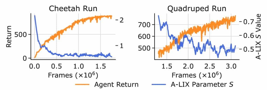
Intuitively, the value of $s$ should decrease throughout training as the useful learning signal from the TD-loss becomes stronger. To quantify the level of discontinuity in the features and their gradients,the authors defined the expected squared local discontinuity of $\mathbf{z}$ in any spatial direction:

\[D(\nabla \mathbf{z})_{ijc} \approx \mathbb{E}_{\mathbf{v} \sim S^1} \left[ \left( \frac{\partial \nabla \mathbf{z}_{ijc}}{\partial \mathbf{v}}\right)^2 \right]\]

where $S^n$ is $n$-dimensional hypersphere and practically estimated via MC sampling. Then, each value in $D(\nabla \mathbf{z})$ is normalized by its squared input and average over all the feature positions:

\[\mathrm{ND}(\nabla \mathbf{z}) = \frac{1}{C \times H \times W} \sum_{c=1}^C \sum_{j=1}^H \sum_{i=1}^W \frac{D(\nabla \mathbf{z})_{ijc} }{\nabla \mathbf{z}_{ijc}^2}\]

and this metric is named as normalized discontinuity score. It can be further stabilized using $\log$ function:

\[\widetilde{\mathrm{ND}}(\nabla \nabla \mathbf{z}) = \sum_{c=1}^C \sum_{j=1}^H \sum_{i=1}^W \log \left(1 + \frac{D(\nabla \mathbf{z})_{ijc} }{\nabla \mathbf{z}_{ijc}^2}\right)\]

Then the scale parameter $s$ adaptively decreases using gradient descent to minimize the following dual objective:

\[\underset{s \in \mathbb{R}}{\arg \min} \left( - s \times \mathbb{E}_{\hat{\mathbf{z}}} \left[ \widetilde{\mathrm{ND}}(\nabla \hat{\mathbf{z}}) - \overline{\mathrm{ND}} \right] \right)\]

$\mathbf{Fig\ 12.}$ A-LIX’s $s$ parameter evolution during training (Cetin et al. 2022)

Scaling Replay Ratios

Update-to-data (UTD) ratio, also known as replay ratio, denotes the number of model updates performed relative to the actual interactions with the environment. While increasing the number of updates for a fixed count of environment interactions seems a logical approach to enhance sample efficiency and performance, empirical reports indicate that simply raising the UTD ratio can actually impair performance.

$\mathbf{Fig\ 13.}$ Simply scaling UTD ratio of SAC even performs worse (D’Oro et al. 2023)

Recent algorithms, such as REDQ (Chen et al. ICLR 2021), DroQ (Hiraoka et al. ICLR 2021), and SR-SPR (D’Oro et al. ICLR 2023), have developed strategies to boost sample efficiency by increasing the replay ratio per environment sample without degrading performance.

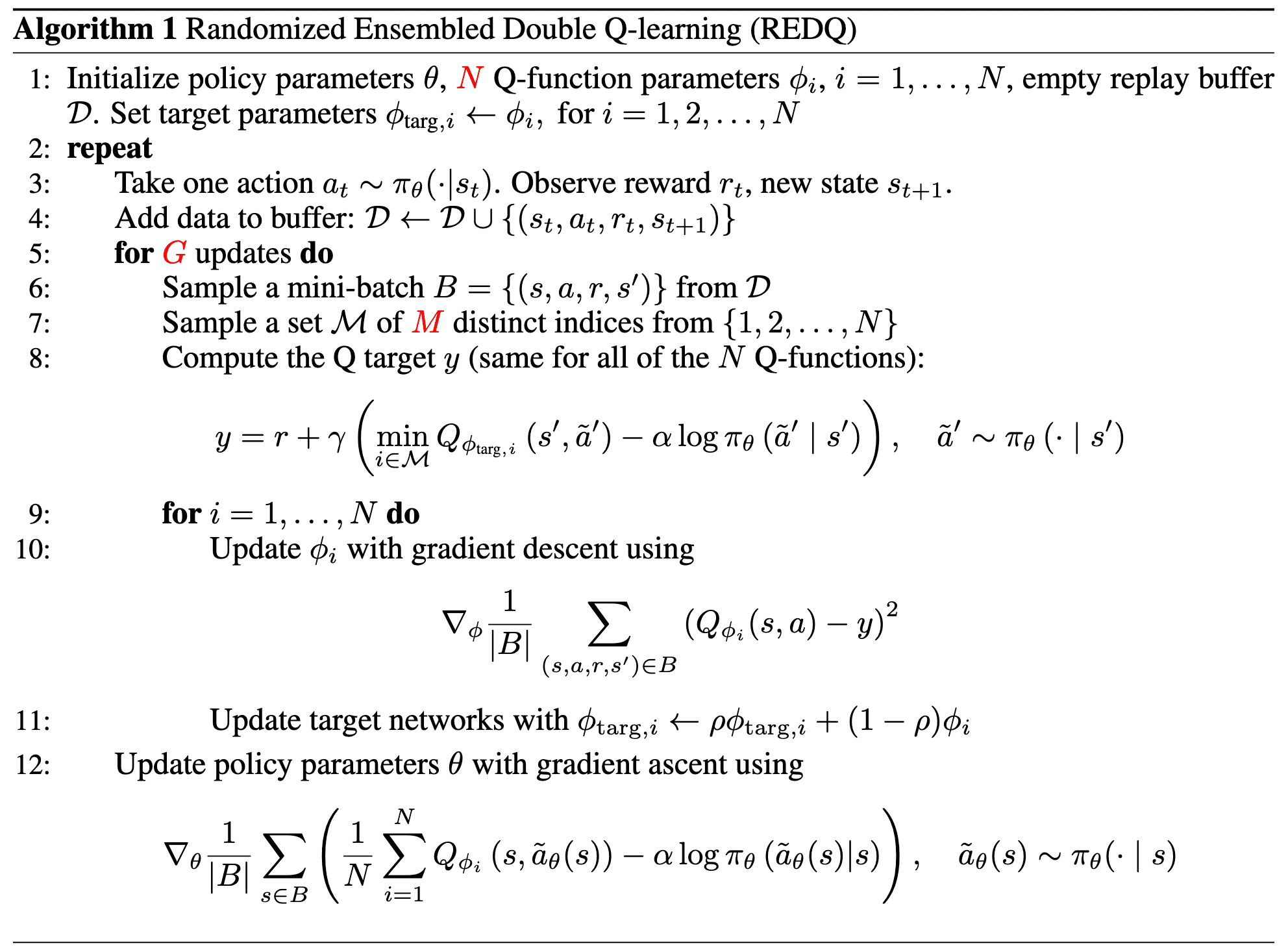
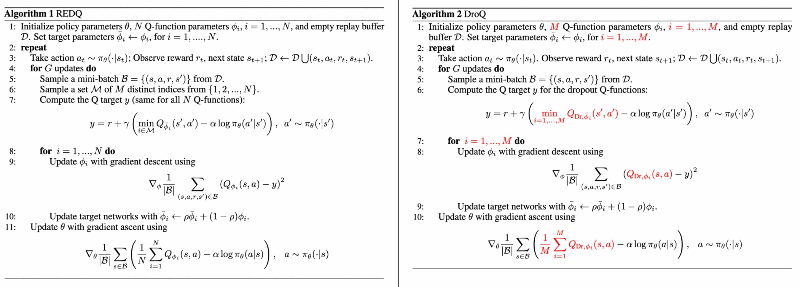
Randomized Ensembled Double Q-Learning (REDQ)

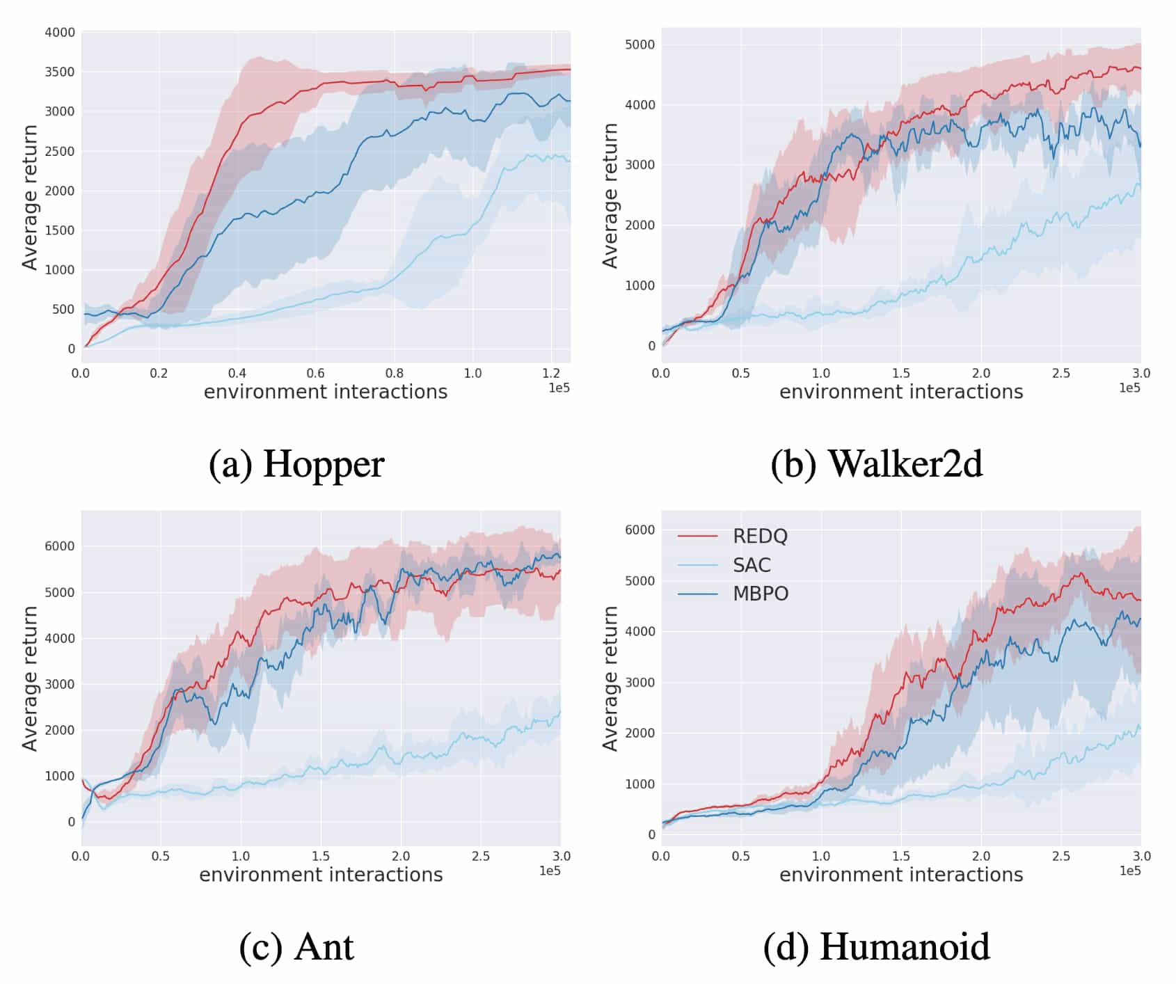
In high UTD ratios, Chen et al. ICLR 2021 argued that the accumulation of estimation bias in the learned Q function’s over multiple update steps can destabilizes learning, even when using the clipped double-Q trick. To more effectively address this bias, they proposed increasing the number of Q-networks from two to an ensemble of $10$. Their method, called Randomized Ensembled Double Q-Learning (REDQ), enables stable training at high replay ratios up to $20$ and achieves $3 \sim 8 \times$ better sample efficiency than the SAC baseline.

$\mathbf{Fig\ 14.}$ REDQ compared to MBPO and SAC when $\mathrm{UTD} = 20$ (Chen et al. 2021)

REDQ uses an ensemble of $N$ Q-networks to control variance:

\[Q_\phi (\mathbf{s}, \mathbf{a}) \equiv \frac{1}{N} \sum_{i=1}^N Q_{\phi_i} (\mathbf{s}, \mathbf{a})\]

and in-target minimization across a random subset $\mathcal{M}$ of these $N$ Q-functions from the ensemble to reduce over-estimation bias:

\[r (\mathbf{s}, \mathbf{a}) + \gamma \max_{\mathbf{a}^\prime \in \mathcal{A}} \min_{j \in \mathcal{M}} Q_{\phi_\texttt{target}, j} (\mathbf{s}^\prime, \mathbf{a}^\prime)\]

$\color{red}{\mathbf{Thm.}}$ $M$ can control the expected estimation bias
For the true Q-value $Q^\pi$, let $Q_{\phi_i} - Q^\pi$ be the pre-update estimation bias for $i$-th Q-funtion and define the post-update estimation bias $Z_{M, N}$: $$ \begin{aligned} Z_{M, N} & \triangleq r (\mathbf{s}, \mathbf{a}) +\gamma \max _{\mathbf{a}^{\prime} \in \mathcal{A}} \min_{j \in \mathcal{M}} Q_{\phi_j}\left(\mathbf{s}^{\prime}, \mathbf{a}^{\prime}\right)-\left( r(\mathbf{s}, \mathbf{a})+\gamma \max_{\mathbf{a}^{\prime} \in \mathcal{A}} Q^\pi\left(\mathbf{s}^{\prime}, \mathbf{a}^{\prime}\right)\right) \\ & =\gamma\left(\max_{\mathbf{a}^{\prime} \in \mathcal{A}} \min_{j \in \mathcal{M}} Q_{\phi_j}\left(\mathbf{s}^{\prime}, \mathbf{a}^{\prime}\right)-\max_{\mathbf{a}^{\prime} \in \mathcal{A}} Q^\pi\left(\mathbf{s}^{\prime}, \mathbf{a}^{\prime}\right)\right) \end{aligned} $$ Therefore, if $\mathbb{E} [Z_{M, N}] > 0$, then the expected post-update bias is positive and there is a tendency for over-estimation accumulation; and if $\mathbb{E}[Z_{M,N}] < 0$, then there is a tendency for under-estimation accumulation. Then, the following statements hold:

1. For any fixed $M$, $\mathbb{E} [Z_{M, N}]$ does not depend on $N$.
2. $\mathbb{E} [Z_{1, N}] \geq 0$ for all $N \geq 1$.
3. $\mathbb{E} [Z_{M+1, N}] \leq \mathbb{E} [Z_{M, N}]$ for any $M < N$.

$\mathbf{Proof.}$

1. For any fixed $M$, $\mathbb{E} [Z_{M, N}]$ does not depend on $N$

Let \(\mathcal{M}_1\) and \(\mathcal{M}_2\) be two subsets of \(\mathcal{N} = \{ 1, \cdots, N \}\) of size $M$. Since \(\{ Q_{\phi_j} (\mathbf{s}, \mathbf{a}) \}_{j=1}^N\) are i.i.d for any $\mathbf{a} \in \mathcal{A}$, \(\min_{j \in \mathcal{M}_1} Q_{\phi, j} (\mathbf{s}, \mathbf{a})\) and \(\min_{j \in \mathcal{M}_2} Q_{\phi, j} (\mathbf{s}, \mathbf{a})\) are identically distributed. Moreover, since \(Q_{\phi_j} (\mathbf{s}, \mathbf{a})\) are independent for all $\mathbf{a} \in \mathcal{A}$ and $1 \leq j \leq N$, \(\{ \min_{j \in \mathcal{M}} Q_{\phi_j} (\mathbf{s}, \mathbf{a}) \}_{\mathbf{a} \in \mathcal{A}}\) are independent for any $\mathcal{M} \subset \mathcal{N}$.

With these fact, we can prove that \(\max_\mathbf{a} \min_{j \in \mathcal{M}_1} Q_{\phi_j} (\mathbf{s}, \mathbf{a})\) with cdf $F_1$ and \(\max_\mathbf{a} \min_{j \in \mathcal{M}_2} Q_{\phi_j} (\mathbf{s}, \mathbf{a})\) with cdf $F_2$ are identically distributed:

\[\begin{aligned} F_1(x) & =\mathbb{P}\left(\max_\mathbf{a} \min _{j \in \mathcal{M}_1} Q_{\phi_j}(\mathbf{s}, \mathbf{a}) \leq x\right)=\mathbb{P}\left(\bigcap_{\mathbf{a} \in \mathcal{A}}\left\{\min _{i \in \mathcal{M}_1} Q_{\phi_j}(\mathbf{s}, \mathbf{a}) \leq x\right\}\right) \\ & =\prod_{\mathbf{a} \in \mathcal{A}} \mathbb{P}\left(\min _{j \in \mathcal{M}_1} Q_{\phi_j}(\mathbf{s}, \mathbf{a}) \leq x\right)=\prod_{\mathbf{a} \in \mathcal{A}} \mathbb{P}\left(\min _{j \in \mathcal{M}_2} Q_{\phi_j}(\mathbf{s}, \mathbf{a}) \leq x\right) \\ & =\mathbb{P}\left(\max_\mathbf{a} \min _{j \in \mathcal{M}_2} Q_{\phi_j}(\mathbf{s}, \mathbf{a}) \leq x\right)=F_2(x) \end{aligned}\]

Then we obtain:

\[\begin{aligned} \mathbb{E}\left[Z_{M, N}\right] & =\gamma \mathbb{E}\left[\left(\max_\mathbf{a} \min _{j \in \mathcal{M}} Q_{\phi_j} (\mathbf{s}, \mathbf{a})-\max_\mathbf{a} Q^\pi(\mathbf{s}, \mathbf{a})\right)\right] \\ & =\gamma \mathbb{E}\left[\frac{1}{\binom{N}{M}} \sum_{\substack{\mathcal{M} \subset \mathcal{N} \\ \vert \mathcal{M} \vert = M}} \max_\mathbf{a} \min _{j \in \mathcal{M}} Q_{\phi_j} (\mathbf{s}, \mathbf{a})\right]-\gamma \max_\mathbf{a} Q^\pi(\mathbf{s}, \mathbf{a}) \\ & =\gamma\left(\mathbb{E}\left[\max_\mathbf{a} \min _{1 \leq j \leq M} Q_{\phi_j} (\mathbf{s}, \mathbf{a})\right]-\max_\mathbf{a} Q^\pi(\mathbf{s}, \mathbf{a})\right) \end{aligned}\]

which does not depend on $N$.

2. $\mathbb{E} [Z_{1, N}] \geq 0$ for all $N \geq 1$

It follows from the first statement:

\[\mathbb{E}\left[Z_{1, N}\right] = \gamma \left( \mathbb{E} [\max_{\mathbf{a} \in \mathcal{A}} Q_{\phi_1} (\mathbf{s}, \mathbf{a})] - \max_{\mathbf{a} \in \mathcal{A}} Q^\pi (\mathbf{s}, \mathbf{a}) \right) \geq 0\]

since $\mathbb{E} [\max_{\mathbf{a}} Q_{\phi_1} (\mathbf{s}, \mathbf{a})] \geq \mathbb{E} [Q_{\phi_1} (\mathbf{s}, \mathbf{a})]$.

3. $\mathbb{E} [Z_{M+1, N}] \leq \mathbb{E} [Z_{M, N}]$ for any $M < N$

Since $\max_{\mathbf{a}} \min_{1 \leq j \leq M} Q_{\phi_j} (\mathbf{s}, \mathbf{a}) \geq \max_{\mathbf{a}} \min_{1 \leq j \leq M+1} Q_{\phi_j} (\mathbf{s}, \mathbf{a})$:

\[\begin{aligned} \mathbb{E}\left[Z_{M, N}\right] & =\gamma\left(\mathbb{E}\left[\max_{\mathbf{a}} \min _{1 \leq j \leq M} Q_{\phi_j} (\mathbf{s}, \mathbf{a})\right]-\max_{\mathbf{a}} Q^\pi(\mathbf{s}, \mathbf{a})\right) \\ & \geq \gamma\left(\mathbb{E}\left[\max_{\mathbf{a}} \min _{1 \leq j \leq M+1} Q_{\phi_j} (\mathbf{s}, \mathbf{a})\right]-\max_{\mathbf{a}} Q^\pi(\mathbf{s}, \mathbf{a})\right)=\mathbb{E}\left[Z_{M+1, N}\right] \end{aligned}\] \[\tag*{$\blacksquare$}\]

$\color{red}{\mathbf{Thm.}}$ $N$ can reduce the variance of the target
Consider the weighted variant of REDQ which calculate the target by taking the expected value over all possible subsets $\mathcal{M}$, instead of choosing a random set $\mathcal{M}$ of size $M$ in the target: $$ Y_{M, N} = r(\mathbf{s}, \mathbf{a}) + \gamma \frac{1}{\binom{N}{M}} \sum_{\substack{\mathcal{M} \subset \mathcal{N} \\ \vert \mathcal{M} \vert = M}} \max_{\mathbf{a}^\prime \in \mathcal{A}} \min_{j \in \mathcal{M}} Q_{\phi_j} (\mathbf{s}^\prime, \mathbf{a}^\prime) $$ Then, the following inequality holds: $$ \mathrm{Var} (Y_{M, N}) \leq f_M (N) $$ for some function $f_M (N)$ satisfying $$ \lim_{N \to \infty} \frac{f_M (N)}{M^2 \mathrm{Var} (Y_{M, N}) / N} = 1 $$ Consequently: $$ \lim_{N \to \infty} \mathrm{Var} (Y_{M, N}) = 0 $$ However, in practice, some variance in the target may be beneficial in reducing overfitting or help exploration. To retian that variance, the practical implementation of REDQ keeps $N$ finite and utilizes the unweighted scheme.

$\mathbf{Proof.}$

For convenience, define $Y_\mathcal{M} = \max_{\mathbf{a}^\prime}\min_{j \in \mathcal{M}} Q_{\phi_j} (\mathbf{s}^\prime, \mathbf{a}^\prime)$. Suppose $N > 2M$.

\[\begin{aligned} \mathrm{Var}(Y_{M, N}) &= \frac{\gamma^2}{\binom{N}{M}^2} \mathrm{Var} \left(\sum_{\substack{\mathcal{M} \subset \mathcal{N} \\ \vert \mathcal{M} \vert = M}} Y_B \right) \\ &= \frac{\gamma^2 (M!)^2}{\left(\Pi_{i=0}^{M-1}(N-i)\right)^2} \left[\sum_{B \subset \mathcal{N}} \mathrm{Var}(Y_B) + 2\cdot \sum_{\substack{\mathcal{M}_1, \mathcal{M}_2 \subset \mathcal{N} \\ \mathcal{M}_1 \neq \mathcal{M}_2}} \mathrm{Cov}(Y_{\mathcal{M}_1}, Y_{\mathcal{M}_2}) \right] \end{aligned}\]

Let \(A = \sum_{\substack{\mathcal{M}_1, \mathcal{M}_2 \subset \mathcal{N} \\ \mathcal{M}_1 \neq \mathcal{M}_2}} \mathrm{Cov}(Y_{\mathcal{M}_1}, Y_{\mathcal{M}_2})\), which consists of

\[\begin{aligned} \binom{\binom{N}{M}}{2} &= \frac{1}{2} \cdot \frac{N!}{(N-M)!M!}\cdot\bigg(\frac{N!}{(N-M)!M!} - 1\bigg) \\ &= \frac{1}{2(M!)^2}\cdot \Pi_{i=0}^{M-1}(N-i)^2 - \frac{N!}{2\cdot M!(N-M)!} \end{aligned}\]

terms. $\binom{\binom{N}{M}}{2}$ can be seen as a polynomial function of $N$ with degree $2M$. That is, the coefficient for the term $N^{2M}$ is $\frac{1}{2(M!)^2}$. Similarly, the coefficient for the term $N^{2M-1}$ is $\frac{1}{2(M!)^2} \cdot (-2\sum_{i=0}^{M-1}i)$.

Note that \(Y_{\mathcal{M}_1}\) and \(Y_{\mathcal{M}_2}\) are independent if \(\mathcal{M}_1 \cap \mathcal{M}_2 = \varnothing\). The total number of different pairs \((\mathcal{M}_1, \mathcal{M}_2)\) such that \(\mathcal{M}_1 \cap \mathcal{M}_2 = \varnothing\) is

\[\begin{equation*} \binom{N}{2M} \cdot \binom{2M}{M} \cdot \frac{1}{2} = \frac{1}{2(M!)^2}\cdot\frac{N!}{(N-2M)!} = \frac{1}{2(M!)^2}\cdot\Pi_{i=0}^{2M-1}(N-i) \end{equation*}\]

This is again a polynomial function of $N$ with degree $2M$. The coefficient of the term $N^{2M}$ is $\frac{1}{2(M!)^2}$. The coefficient of the term $N^{2M-1}$ is $\frac{1}{2(M!)^2} \cdot (-\sum_{i=0}^{2M-1}i)$. So the number of non-zero terms in $A$ is at most

\[\begin{aligned} &\frac{1}{2(M!)^2}\cdot \Pi_{i=0}^{M-1}(N-i)^2 - \frac{N!}{2\cdot M!(N-M)!} - \frac{1}{2(M!)^2}\cdot\Pi_{i=0}^{2M-1}(N-i) \\ = &\frac{M^2}{2(M!)^2} \cdot N^{2M-1} + O(N^{2M-2}) \end{aligned}\]

Using Cauchy-Schwarz inequality, for any $\mathcal{M}_1, \mathcal{M}_2 \subset \mathcal{N}$:

\[\begin{equation*} \mathrm{Cov}(Y_{\mathcal{M}_1}, Y_{\mathcal{M}_2}) \le \sqrt{ \mathrm{Var}(Y_{\mathcal{M}_1})\cdot \mathrm{Var}(Y_{\mathcal{M}_2})} = \mathrm{Var} (Y_{M, N}) \end{equation*}\]

Therefore:

\[\begin{equation*} A \leq \left[\frac{M^2}{2(M!)^2} \cdot N^{2M-1} + O(N^{2M-2}) \right] \times \mathrm{Var} (Y_{M, N}) \end{equation*}\]

which implies

\[\begin{aligned} \mathrm{Var}(Y_{M,N}) &= \frac{\gamma^2 (M!)^2}{\left(\Pi_{i=0}^{M-1}(N-i)\right)^2}\left[\sum_{B \subset \mathcal{N}} \mathrm{Var}(Y_B) + 2\cdot \sum_{\substack{\mathcal{M}_1, \mathcal{M}_2 \subset \mathcal{N} \\ \mathcal{M}_1 \neq \mathcal{M}_2}} \mathrm{Cov}(Y_{\mathcal{M}_1}, Y_{\mathcal{M}_2}) \right] \\ & = \frac{\gamma^2 (M!)^2}{\left(\Pi_{i=0}^{M-1}(N-i)\right)^2}\left[\sum_{B \subset \mathcal{N}} \mathrm{Var}(Y_B) + 2A \right] \\ &\le \gamma^2 \left[M^2 \cdot \frac{N^{2M-1}}{\Pi_{i=0}^{M-1}(N-i)^2} + \mathcal{O} \left(\frac{1}{N^2} \right)\right] \times \mathrm{Var} (Y_{M, N}) \xrightarrow{N \to \infty} 0 \end{aligned}\]

Moreover,

\[\begin{equation*} \lim_{N \to \infty} \frac{M^2 \mathrm{Var} (Y_{M, N})/N}{\left[M^2 \cdot \frac{N^{2M-1}}{\Pi_{i=0}^{M-1}(N-i)^2} + O(\frac{1}{N^2})\right] \mathrm{Var} (Y_{M, N})} = \lim_{N \to \infty} \frac{\Pi_{i=0}^{M-1}(N-i)^2}{N^{2M}} = 1 \end{equation*}\] \[\tag*{$\blacksquare$}\]

$\mathbf{Fig\ 15.}$ Randomized Ensembled Double Q-learning (Chen et al. 2021)

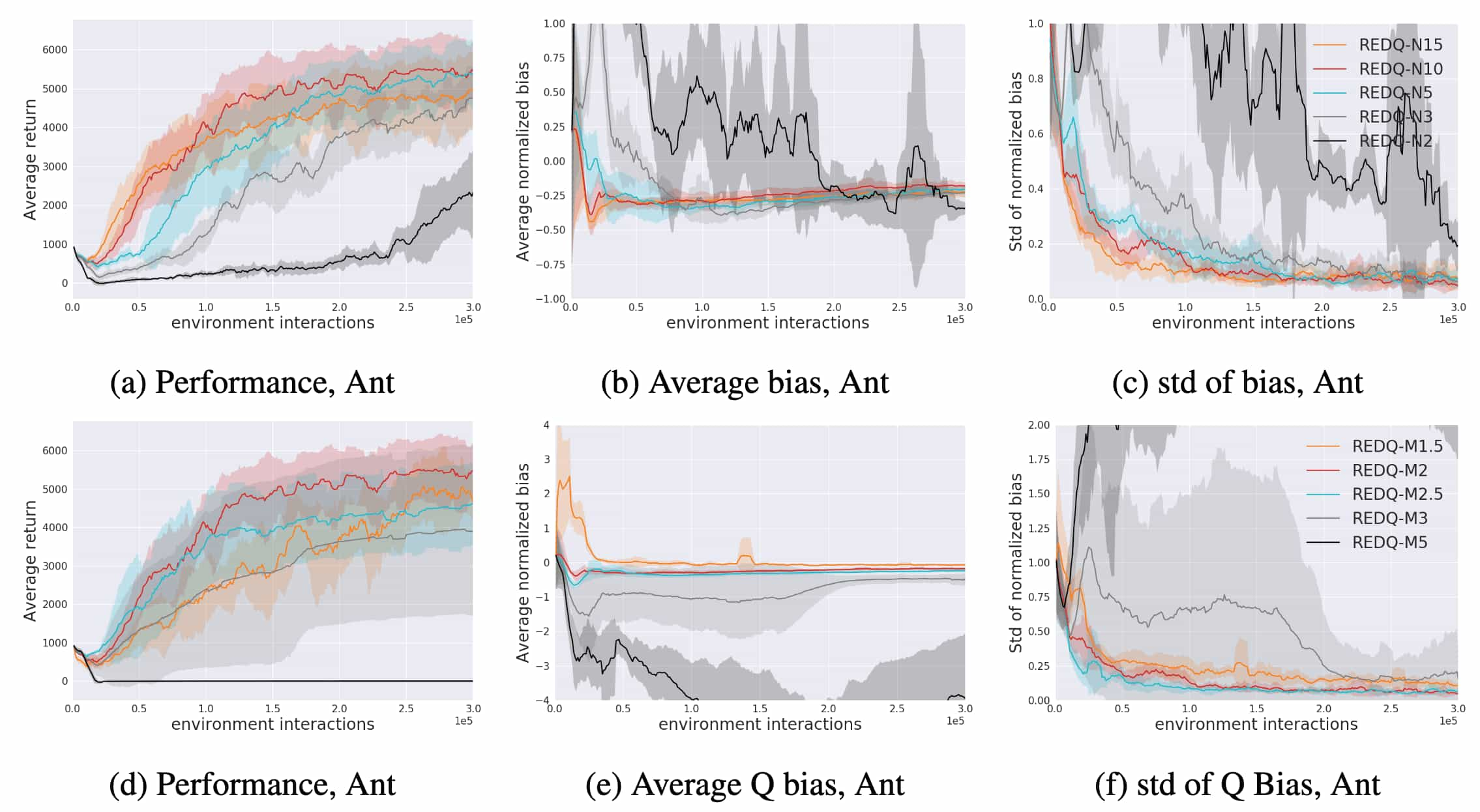
In practice, similar bias trends align with the theoretical insights. When $N = 2$, $3$, $5$, $10$, $15$, the REDQ agent typically achieves a more stable average bias, a reduced standard deviation of bias, and improved performance under high UTD ratios. Furthermore, consistent with the theorem, increasing $M$ reduces the average bias. However, excessively large $M$ values make the Q-estimate overly conservative, introducing a significant negative bias that hinders effective learning.

$\mathbf{Fig\ 16}$ REDQ ablation results for Ant (Chen et al. 2021)

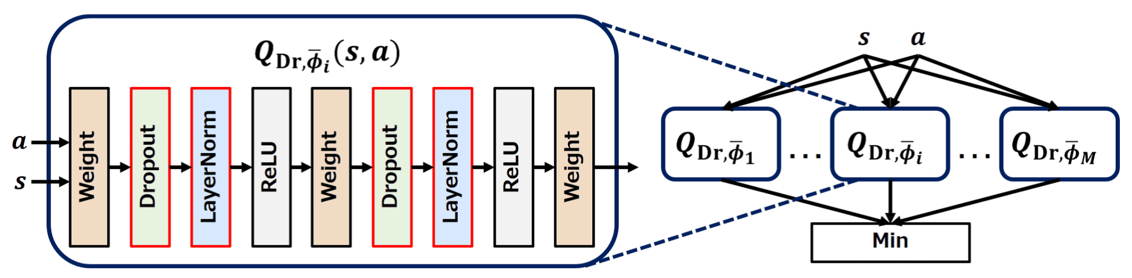
Dropout Q-Functions (DroQ)

Hiraoka et al. ICLR 2021 note that REDQ’s ensemble size, along with its high UTD ratio, makes training computationally expensive. They instead propose using a smaller ensemble of Q functions equipped with Dropout and Layer Normalization to stabilize training in response to the noise introduced by Dropout. Called DroQ, their method is computationally cheaper than REDQ, yet still expensive due to its UTD ratio of $20$.

$\mathbf{Fig\ 17.}$ Dropout Q-function implementation and how dropout Q-functions are used in target (Hiraoka et al. 2022)

Recall that the REDQ utilized the minimum of $M = 2$ ensembles across a random subset $\mathcal{M}$ of $N = 10$ target Q-functions \(Q_{\phi_{\texttt{target}}}\) as a TD-target, to reduce overestimation bias:

\[\begin{aligned} y_t & = r (\mathbf{s}_t, \mathbf{a}_t) + \gamma \left( \min_{j \in \mathcal{M}} Q_{\phi_{\texttt{target}}, j} (\mathbf{s}_{t+1}, \mathbf{a}_\pi) - \alpha \log \pi_\theta (\mathbf{a}_\pi \vert \mathbf{s}_{t+1}) \right) \\ \hat{Q} (\mathbf{s}_t, \mathbf{a}_t) & = \frac{1}{N} \sum_{i=1}^N Q_{\phi, i} (\mathbf{s}_t, \mathbf{a}_t) \end{aligned}\]

DroQ empirically shows that Q-functions $Q_{\texttt{Dr}, \phi}$ equipped with dropout connection and layer normalization enable to choose small $M = N = 2$, simulatenously achieving comparable computational efficiency than REDQ:

\[\begin{aligned} y_t & = r (\mathbf{s}_t, \mathbf{a}_t) + \gamma \left( \color{red}{ \min_{j = 1, \cdots, M} Q_{\texttt{Dr}, \phi_{\texttt{target}}, j} (\mathbf{s}_{t+1}, \mathbf{a}_\pi)} - \alpha \log \pi_\theta (\mathbf{a}_\pi \vert \mathbf{s}_{t+1}) \right) \\ \hat{Q} (\mathbf{s}_t, \mathbf{a}_t) & = \color{red}{\frac{1}{M} \sum_{j=1}^M Q_{\texttt{Dr}, \phi, j} (\mathbf{s}_t, \mathbf{a}_t)} \end{aligned}\]

$\mathbf{Fig\ 18.}$ (Left) REDQ v.s. (Right) DroQ (Hiraoka et al. 2022)

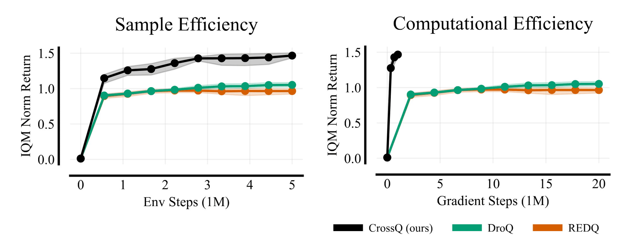
Aside: CrossQ

Both REDQ and DroQ demonstrated that simply increasing the UTD ratio is ineffective due to the Q-value estimation bias in the critic networks. To address this, ensembling techniques were introduced to mitigate bias (explicit ensemble in REDQ and implicit ensemble via dropout in DroQ), which enables increasing the UTD to $20$ critic updates per environment step.

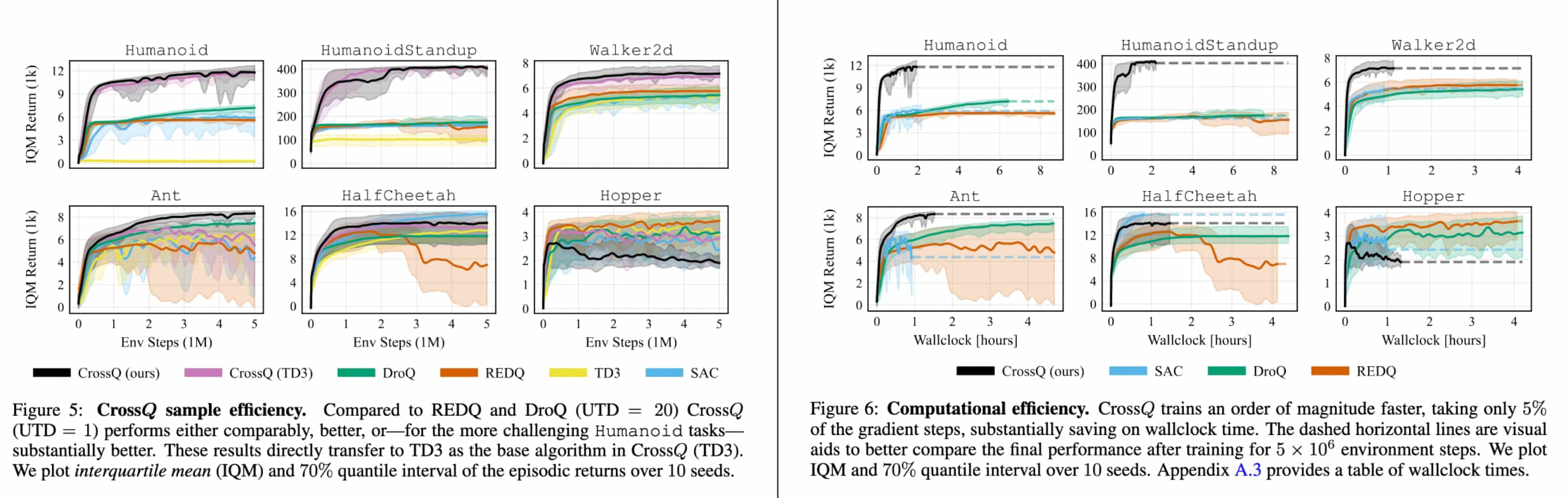
While higher UTD ratios enhance sample efficiency, they come at the cost of increased computational demands, resulting in greater wall-clock time and energy consumption. Bhatt et al. ICLR 2024 proposed CrossQ, a streamlined algorithm that achieves superior performance by crossing out much of the algorithmic complexity. Notably, it leverages Batch Normalization effectively and removes target networks, surpassing the current state-of-the-art in sample efficiency while maintaining a low UTD ratio of $1$.

$\mathbf{Fig\ 19.}$ CrossQ training performance aggregated over environments (Bhatt et al. 2024)

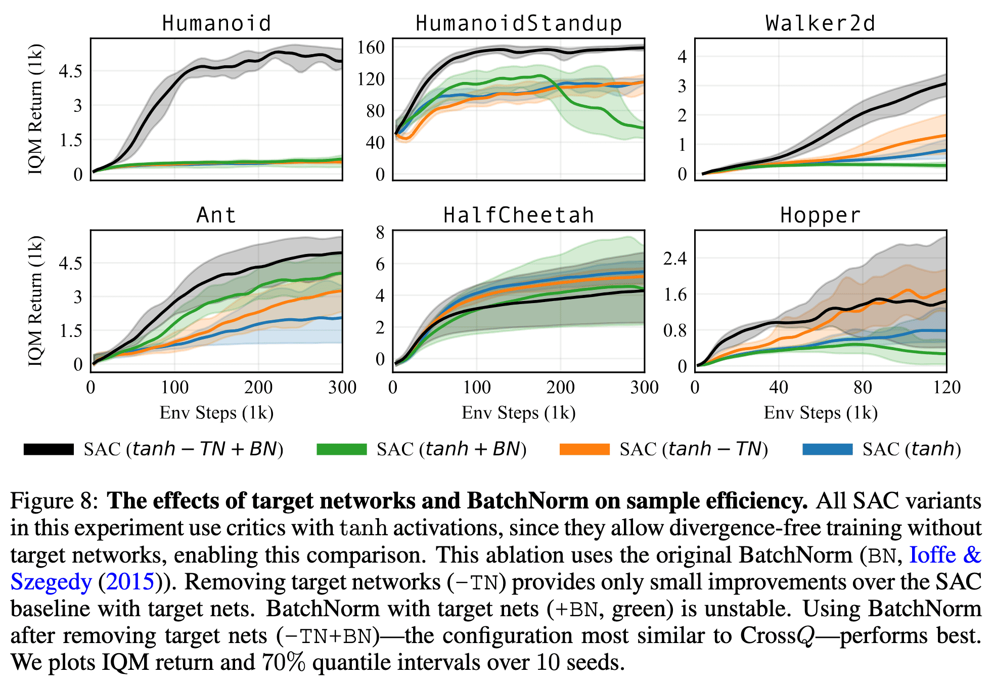
1. Removing Target Network

Target networks, first introduced in the DQN algorithm, stabilize training by explicitly delaying value function updates, albeit at the expense of potentially slowing down online learning. The authors empirically demonstrate that employing bounded activation functions (e.g., $\tanh$) or feature normalization is sufficient to prevent critic divergence in the absence of target networks. In contrast, the common choice of $\text{ReLU}$ without normalization leads to divergence.

2. Batch Renormalization (BRN)

Batch Normalization has not been widely adopted in RL algorithms due to the inherently non-stationary behavior of RL agents. For example, in the critic loss, TD predictions \(Q_\boldsymbol{\theta} (\mathbf{s}_t, \mathbf{a}_t) - (r (\mathbf{s}_t, \mathbf{a}_t) + Q_{\boldsymbol{\theta}^\prime} (\mathbf{s}_{t+1}, \mathbf{a}_{t+1}))\) are calculated for two differently distributed batches of state-action pairs: \((\mathbf{s}_t, \mathbf{a}_t)\) and \((\mathbf{s}_{t+1}, \mathbf{a}_{t+1})\). Here, the next action \(\mathbf{a}_{t+1} \sim \pi_\phi(\mathbf{s}_{t+1})\) is sampled from the current actor, whereas \(\mathbf{a}_t\) originates from the historical behavior of actors.

$\mathbf{Fig\ 20.}$ 2D kernel density estimate of the distributions of $\color{blue}{\mathbf{a}_t}$ and $\color{red}{\mathbf{a}_{t+1}}$. Two action distributions are different, and evolve during training (Bhatt et al. 2024)

Eliminating the target network offers an elegant solution to this issue. By concatenating both batches and passing them through the Q-network in a single forward pass, this ensures consistent normalization across the combined batches:

\[\begin{matrix} \text{SAC} & \text{CrossQ} \\ {\begin{aligned} {\color{magenta}Q_{\boldsymbol{\theta}}}(\mathbf{s}_t,\mathbf{a}_t) &= q_t \\ {\color{magenta}Q_{\boldsymbol{\theta}^\circ}}(\mathbf{s}_{t+1},\mathbf{a}_{t+1}) &= {\color{purple}q_{t+1}^\circ} \end{aligned}} & {\begin{aligned} {\color{cyan}Q_\boldsymbol{\theta}}\left( \begin{bmatrix} \begin{aligned} &\mathbf{s}_t \\ &\mathbf{s}_{t+1} \end{aligned} \end{bmatrix}, \begin{bmatrix} \begin{aligned} &\mathbf{a}_t \\ &\mathbf{a}_{t+1} \end{aligned} \end{bmatrix} \right) = \begin{bmatrix} \begin{aligned} &q_t \\ &q_{t+1} \end{aligned} \end{bmatrix} \end{aligned}} \\ {\begin{aligned} \mathcal{L}_{\color{magenta}{\boldsymbol{\theta}}} &= (q_t - r_t - \gamma\, {\color{purple}q^\circ_{t+1}})^2 \end{aligned}} & {\begin{aligned} \mathcal{L}_{\color{cyan}{\boldsymbol{\theta}}} &= (q_t - r_t - \gamma\,|q_{t+1}|_{\mathtt{sg}})^2 \end{aligned}} \end{matrix}\]

def critic_loss(Q_params, policy_params, obs, acts, rews, next_obs):
    next_acts, next_logpi = policy.apply(policy_params, obs)

    # Concatenated forward pass
    all_q, new_Q_params = Q.apply(Q_params,
        jnp.concatenate([obs, next_obs]), 
        jnp.concatenate([acts, next_acts])
    )
    # Split all_q predictions and stop gradient on next_q
    q, next_q = jnp.split(all_q, 2)
    next_q = jnp.min(next_q, axis=0)   # min over double Q function
    next_q = jax.lax.stop_gradient(next_q - alpha * next_logpi)
    return jnp.mean((q - (rews + gamma * next_q))**2), new_Q_params

This straightforward technique ensures that BatchNorm’s normalization moments are derived from the combined batches, effectively creating a 50/50 mixture of their respective distributions. In practice, the authors utilized Batch ReNormalization (BRN) instead of BatchNorm, as BRN is more resilient to long-term training instabilities caused by minibatch noise:

\[\frac{x - \mu}{\sigma}\]

$\mathbf{Fig\ 21.}$ Removing target networks and adding BatchReNorm that accelerates learning the most (Bhatt et al. 2024)

Experimental Results

CrossQ, a $\text{UTD} = 1$ method, does not use bias-reducing ensembles, high UTD ratios or target networks. Despite this, it achieves its competitive sample efficiency at a fraction of the compute cost of REDQ and DroQ.

$\mathbf{Fig\ 22.}$ Efficiency of CrossQ (Bhatt et al. 2024)

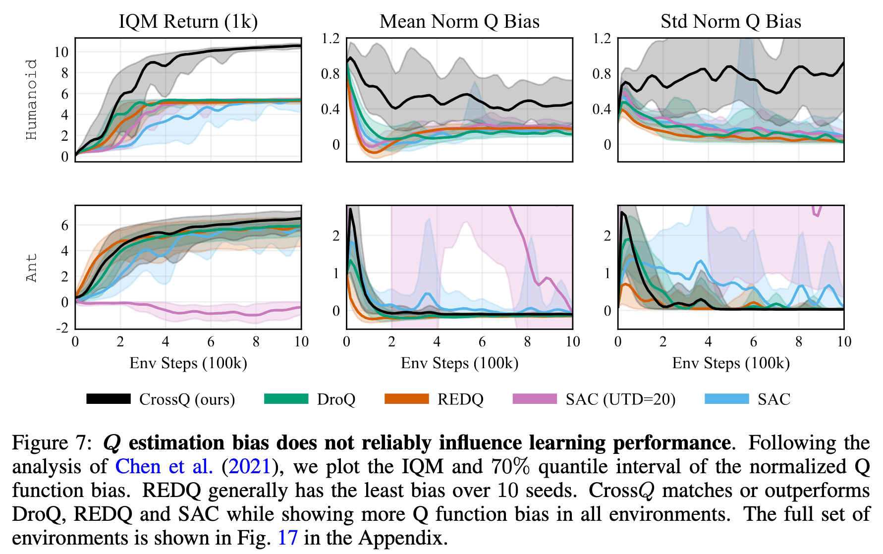
The authors find that REDQ and DroQ indeed have lower bias than SAC and significantly lower bias than SAC with UTD = 20. The results for CrossQ are mixed: while its bias trend shows a lower mean and variance than SAC, in certain environments, its bias exceeds that of DroQ, while in others, it is lower or comparable. REDQ maintains the least bias but achieves returns that are comparable to or worse than CrossQ. Interestingly, CrossQ outperforms despite exhibiting—paradoxically—generally higher Q-estimation bias. This suggests that the relationship between performance and estimation bias is complex, with no clear or direct correlation between the two.

$\mathbf{Fig\ 23.}$ Q estimation bias does not reliably influence learning performance (Bhatt et al. 2024)

Scaled-by-Resetting (SR)

D’Oro et al. ICLR 2023 argue that the loss of plasticity of neural networks to lose their ability to learn and generalize from new information during training has been the main roadblock in achieving better sample efficiency through replay ratio scaling. And they demonstrate that fully or partially resetting the parameters of deep RL agents at higher frequencies causes better replay ratio scaling capabilities to emerge.

$\mathbf{Fig\ 24.}$Replay ratio scaling drastically improves sample efficiency (D’Oro et al. 2023)

The authors apply two different reset strategies to two standard continuous control (SAC) and discrete control algorithms (SPR).

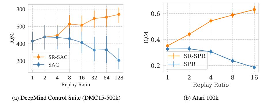
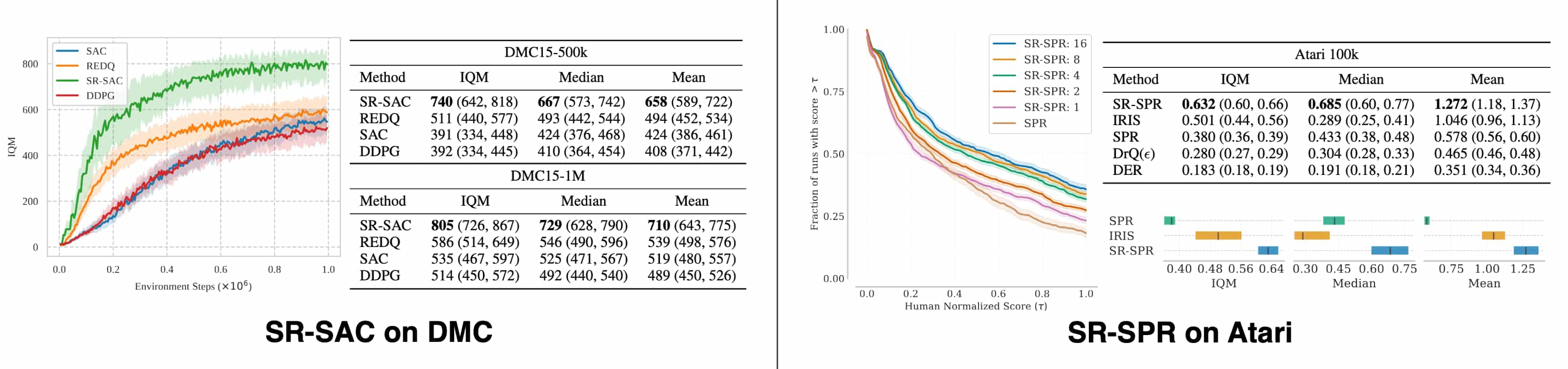
1. SR-SAC
   The parameter of the agent is completely resetted every $2.56 \times 10^6$ of its updates. Note that resets will just occur more often at higher replay ratios in terms of environment step; for example, a reset occurs once every $20000$ interaction steps for replay ratio $128$.
2. SR-SPR
   Similar to Shrink and Perturb (SP), the parameter of the agent's encoder is partially resetted every $40000$ of its updates using interpolation between the previous version and a randomly re-initialized parameter: $$ \theta_t \leftarrow \tau \theta_{t-1} + (1-\tau) \phi \quad \text{ where } \quad \phi \sim \texttt{initializer} $$ with $\tau = 0.8$ by default.

Consequently, SR-SAC and SR-SPR establish a new state-of-the-art result for model-free continuous and discrete control, respectively.

$\mathbf{Fig\ 25.}$ Replay ratio scaling drastically improves sample efficiency (D’Oro et al. 2023)

The importance of online interaction

Changing the replay ratio in a deep RL algorithm can be viewed as a deliberate approach to increasing the proportion on offline training. Specifically, the agent’s parameters are updated a number of times equivalent to the replay ratio before any new data is collected. Therefore, at high replay ratios, the training process begins to resemble offline RL: while the agent retains the capacity to interact with the environment, these interactions occur at a far lower frequency compared to the volume of training. This raises a key question:

What function does the incoming stream of interactions serve?

1. Uniform distribution of the number of offline updates across timesteps is an important factor
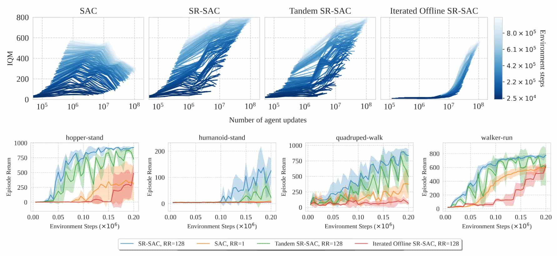
   When the replay ratio $r \geq 1$, the agent performs $r$ updates for each interaction (or data collection) step. Instead, by considering the $\texttt{iterated offline}$ setting that alternates between purely offline updates and data collection phases (e.g. $100000$ data collection steps followed by $100000 \times r$ updates), the authors argue that this uniform distribution of the number of updates across timesteps is a critical determinant in the replay ratio scaling behavior.
   
   Interestingly, the iterated offline RL setting often yields degenerate policies unable to surpass past policies. Favorable replay scaling is observed only when the training regime leans toward the online setting, where update steps remain proportionate to data collection steps.
2. Online interactions as an implicit regularization
   To explore the role of online interactions, the authors designed experiments in a $\texttt{tandem}$ setting where two copies of the same SR-SAC agents, identical apart from the initialization, are created with different roles. The active agent (SR-SAC) collects data and trains using its replay buffer, while the other passive agent (Tandem SR-SAC) trains on the same buffer but cannot interact with the environment to correct its misconceptions.
   
   The results reveal significant behavioral differences between the active agent (blue curve) and the passive agent (green curve), particularly in hopper-stand and quadruped-walk. After a reset, both agents experience an initial performance surge due to high replay ratio training. However, while the active agent's performance stabilizes over time, the passive agent's performance impairs, highlighting the stabilizing influence of online interactions.

$\mathbf{Fig\ 26.}$ Scaling behavior of SAC, SR-SAC and its tandem and iterated offline variations (D’Oro et al. 2023)

Requirements for replay ratio scaling

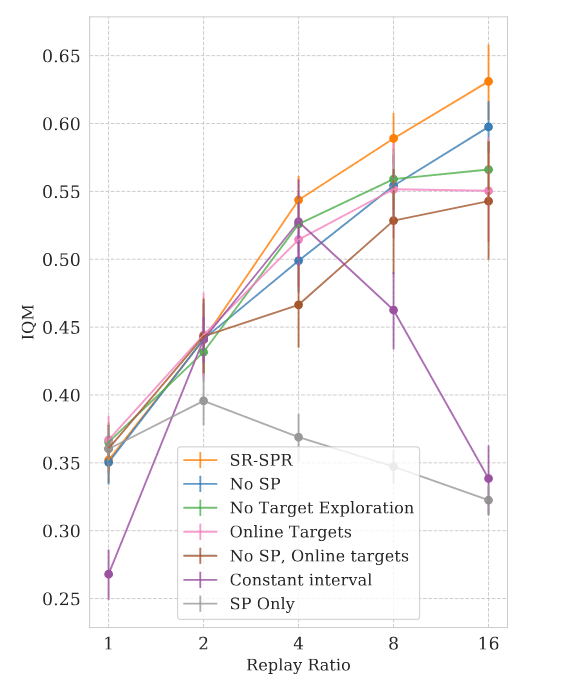
Achieving robust replay ratio scaling for SR-SPR requires more complex design decisions than SR-SAC, due to SR-SPR’s shorter training period and more complex function approximation.

1. Shrink-and-Perturb (SP)
   Applied to the encoder to mitigate plasticity loss and yields a small but consistent improvement (e.g., IQM +0.04 at replay ratio > 4). However, alone is not sufficient; resetting final layers remains crucial because they are most responsible for plasticity loss.
2. Target Network
   Target network was the primary driver of improved replay ratio scaling by providing better action selection (stabilizing effect by target network on optimization is secondary). Removing both SP and the target network scales less effectively at higher replay ratios.

$\mathbf{Fig\ 27.}$ Ablation study on SR-SPR (D’Oro et al. 2023)

Scaling Network Capacities

In contrast to the scalability trend of deep learning networks, conventional practice in continuous deep RL has relied on small network architectures with the primary focus on algorithmic improvements, and some prior researches suggests that naive model capacity scaling can degrade performance, since large number of samples might be needed to gather enough experience so as to determine the long-term effect of different action choices as well as train such large networks effectively.

$\mathbf{Fig\ 28.}$ Scaling network widths for both ResNet and CNN architectures (Schwarzer et al. 2023)

BBF (Schwarzer et al. ICML 2023) and BRO (Nauman et al. 2024) attempt to achieve a significant performance improvements in continuous control by sample-efficiently scaling parameter and replay buffer.

Bigger, Better, Faster (BBF)

Bigger, Better, Faster (BBF) introduced by Schwarzer et al. ICML 2023 explores the interplay between scaling model capacity and integrating domain-specific RL enhancements. Building upon the SR-SPR agent, their investigation culminates in the Bigger, Better, Faster (BBF)</stronb> agent, which achieves super-human performance on Atari 100K in approximately six hours on a single GPU.

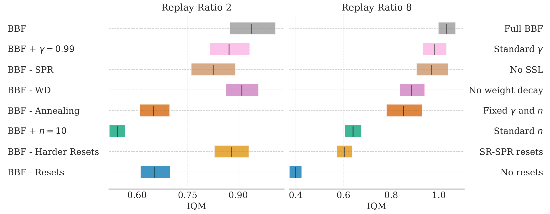
Key Enhancements in BBF

1. Harder Resets
   Recall that SR-SPR employs a shrink-and-perturb reset that convolutional layers were perturbed $20\%$ towards a random target, while later layers were fully reset to a random initialization. The authors find that more regularizing the large model by perturbing $50\%$ yields better performance.
2. Receding update horizon
   BBF exponentially decreases its number of update horizon ($n$-step) from $10$ to $3$ over the first 10K gradient steps following each network reset. This is because larger values of $n$-step leads to faster convergence, and decreasing $n$ mitigates its higher asymptotic errors with respect to the optimal value function.
3. Increasing discount factor
   The authors increase $\gamma$ from $\gamma_1 = 0.97$ to $\gamma_2 = 0.997$ following the exponential scehdule. Note that increasing $\gamma$ has the effect of progressively giving more weights to delayed rewards.
4. Weight decay
   to curb statistical overfitting at high UTD ratio, BBF incorporates AdamW optimizer with weight decay.
5. Removing NoisyNets
   Recall that SPR employs DQN head for its Q learning, containing NoisyNets that introduce Gaussian noises into its parameter. The authors find that this did not improve performance due to over-exploration.

$\mathbf{Fig\ 29.}$ Evaluating the impact of removing the various components that make up BBF with RR=2 and RR=8 (Schwarzer et al. 2023)

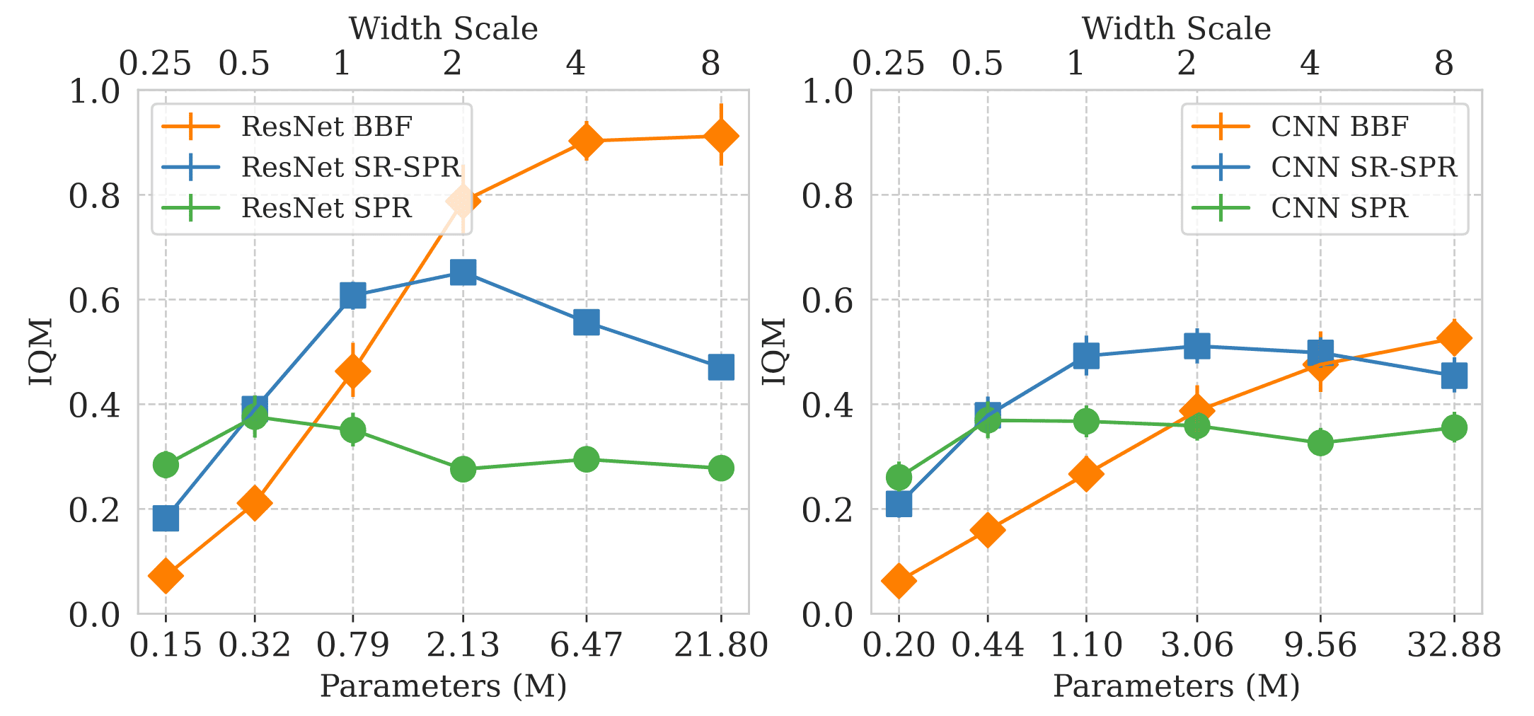
Building upon these design choices, BBF’s performance continues to improve as network capacity scales by increasing layer width.

$\mathbf{Fig\ 30.}$ Scaling network widths for both ResNet and CNN architectures (Schwarzer et al. 2023)

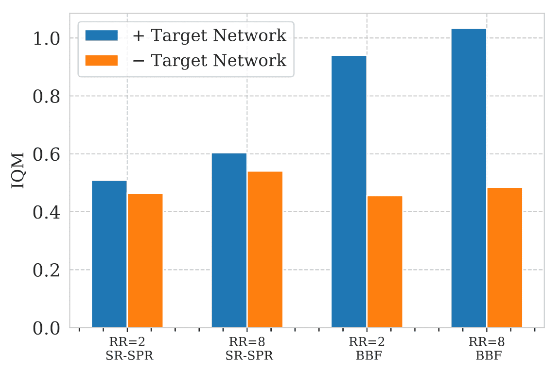
Importance of Target Network for Scaling Network

While some prior works, such as CrossQ, opted to discard target networks, the authors demonstrate that incorporating a target network remains a crucial component across all replay ratios, especially when scaling network capacity.

$\mathbf{Fig\ 31.}$ Comparison of BBF and SR-SPR at replay ratios 2 and 8 with and without EMA target networks (Schwarzer et al. 2023)

Bigger, Regularized, Optimistic (BRO)

Nauman et al. NeurIPS 2024 investigates the advantages and computational trade-offs associated with scaling along two key dimensions: the number of network parameters and the UTD ratios. Bigger, Regularized, Optimistic (BRO) is the culmination of their research, integrating Soft Actor-Critic (SAC) with the BroNet architecture to enhance critic scaling while enforcing robust regularization techniques and fostering optimistic exploration.

Key Enhancements in BRO

1. Bigger
   BRO employs an expanded critic network, featuring approximately 5 million parameters—roughly seven times the size of standard SAC models. Additionally, it adopts an elevated UTD ratio, with a default replay ratio of $RR = 10$, while a more streamlined BRO (Fast) variant operates at $RR = 2$.
2. Regularized
   At the core of BRO lies the BroNet architecture, carefully designed to reinforce regularization and enhance stability. This is achieved through Layer Normalization applied after each dense layer, combined with weight decay and periodic full-parameter resets.
   

   
   

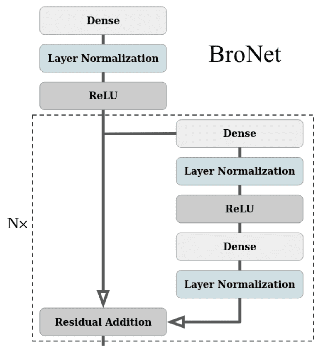
   $\mathbf{Fig\ 32.}$ BroNet architecture employed for actor and critic (Nauman et al. 2024)

3. Optimistic
   BRO uses dual policy optimistic exploration and non-pessimistic (removing clipped double Q-learning) quantile Q-value estimation for balancing exploration and exploitation.

$\mathbf{Fig\ 33.}$ Impact of removing various BRO components on its performance (Nauman et al. 2024)

Building upon these design choices, BRO’s performance continues to improve as network capacity expands through increased layer width, alongside the scaling of the UTD ratio.

$\mathbf{Fig\ 34.}$ The left figure shows performance scaling with increasing replay ratios (shapes) and model sizes (colors).
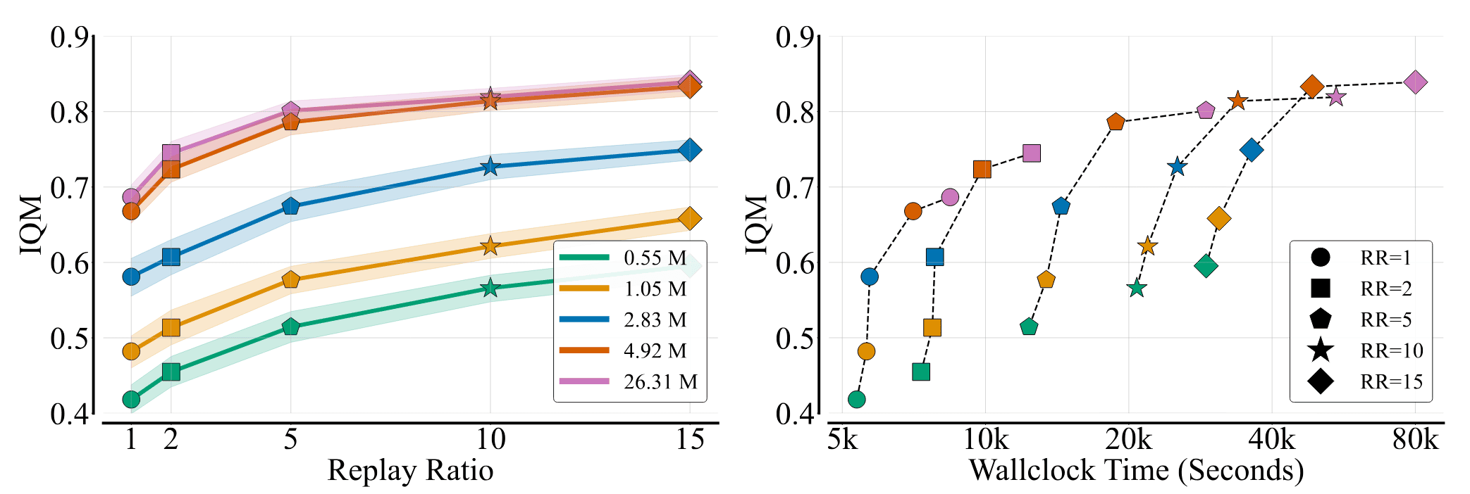
The right figure examines the tradeoff between performance and computational cost when scaling replay ratios versus critic model sizes. (Nauman et al. 2024)

Analysis

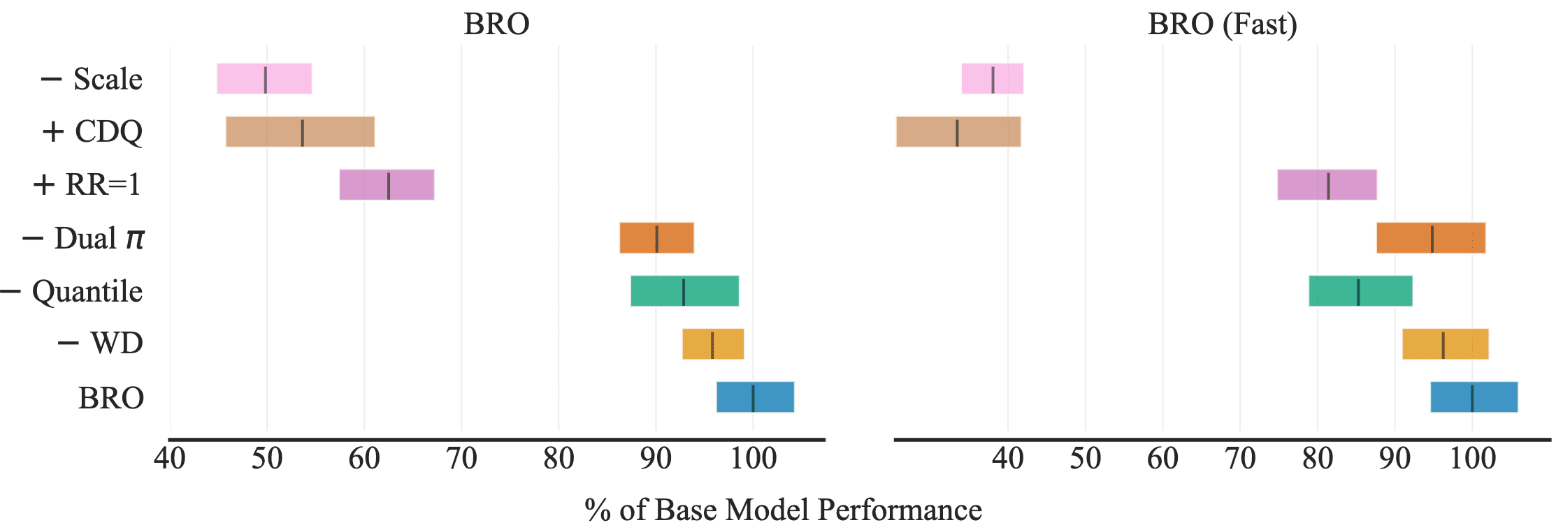
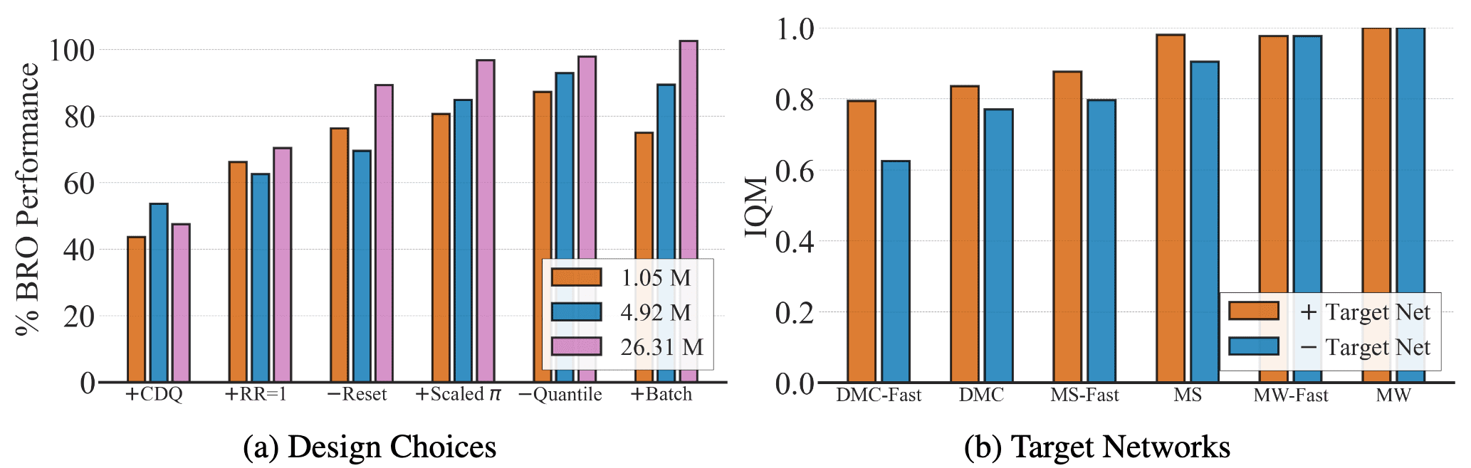
The authors’ key findings are as follows:

1. Algorithmic improvements matter less at scale
   The effectiveness of algorithmic enhancements diminishes as model size increases. While such techniques significantly boost performance for smaller models, they offer little to no gains for the largest models. However, full-parameter resets remain beneficial; in fact, the largest model without resets nearly matches the performance of BRO with resets.
2. Target networks provide small but notable benefits
   Although target networks double memory costs—a significant drawback for large models—they offer a modest yet consistent performance improvement. However, the impact varies considerably across different benchmarks and environments.

$\mathbf{Fig\ 35.}$ The importance of BRO componenets and target network dependent on the critic model size and environments. (Nauman et al. 2024)

References

[1] Cetin et al. “Stabilizing Off-Policy Deep Reinforcement Learning from Pixels”, ICML 2022
[2] Chen et al. “Randomized Ensembled Double Q-Learning: Learning Fast Without a Model”, ICLR 2021
[3] Hiraoka et al. “Dropout Q-Functions for Doubly Efficient Reinforcement Learning”, ICLR 2022
[4] Bhatt et al. “Batch Normalization in Deep Reinforcement Learning for Greater Sample Efficiency and Simplicity”, ICLR 2024
[5] D’Oro et al. “Sample-efficient reinforcement learning by breaking the replay ratio barrier”, ICLR 2023
[6] Schwarzer et al. “Bigger, Better, Faster: Human-level Atari with human-level efficiency”, ICML 2023
[7] Nauman et al. “Bigger, Regularized, Optimistic: scaling for compute and sample-efficient continuous control”, NeurIPS 2024 Spotlight