[Representation Learning] The SimCLR Family

SimCLR v1

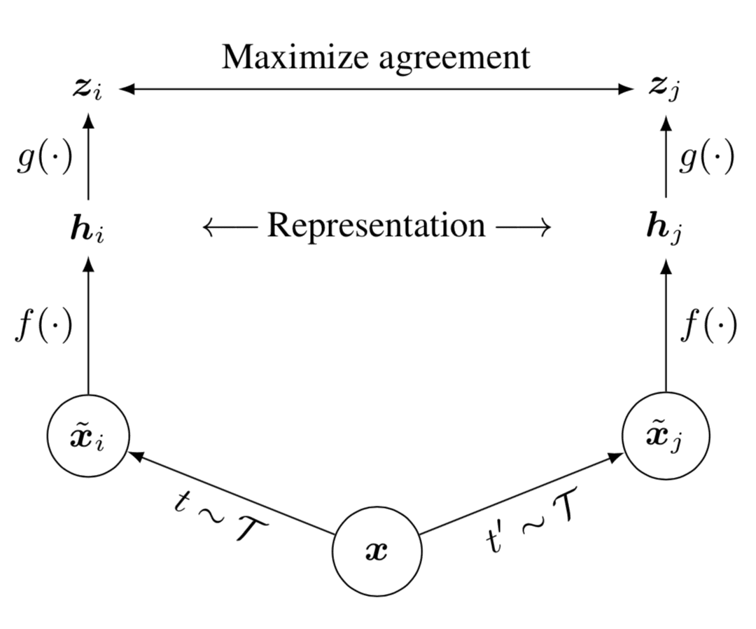
SimCLR, proposed by Chen et al., 2020 provides a simple framework for contrastive learning of visual representations. SimCLR learns representations for visual data by maximizing agreement between differently augmented views of the same sample via a contrastive loss in the latent space.

$\mathbf{Fig\ 1.}$ SimCLR framework (Chen et al., 2020)

1. Create positive pairs
   Randomly sample a minibatch of $N$ examples of $\boldsymbol{x}$ and define the contrastive prediction task on pairs of augmented examples derived from the minibatch, resulting in $2N$ data points. $$ \begin{aligned} \tilde{\boldsymbol{x}}_i = t(\boldsymbol{x}),\quad\tilde{\boldsymbol{x}}_j = t'(\boldsymbol{x}),\quad t, t^\prime \sim \mathcal{T} \end{aligned} $$ where two different data augmentation operators $t, t^\prime$ are sampled from the same family of augmentations $\mathcal{T}$. SimCLR used random crops (with horizontal flips and resize), color distortion, and Gaussian blur. The strengths (e.g., the amount of blur) and compositions of these augmentations impact performance and therefore are typically treated as a hyperparameter.
2. Extract representations from augmented data examples
   Given a positive pair $(\tilde{\boldsymbol{x}}_i, \tilde{\boldsymbol{x}}_j)$, we treat the other $2(N − 1)$ augmented examples within a minibatch as negative examples. The representation is extracted by a base encoder $f(\cdot)$: $$ \begin{aligned} \boldsymbol{h}_i = f(\tilde{\boldsymbol{x}}_i),\quad \boldsymbol{h}_j = f(\tilde{\boldsymbol{x}}_j) \end{aligned} $$ The authors adopt ResNet for $f$.
3. Define the contrastive loss
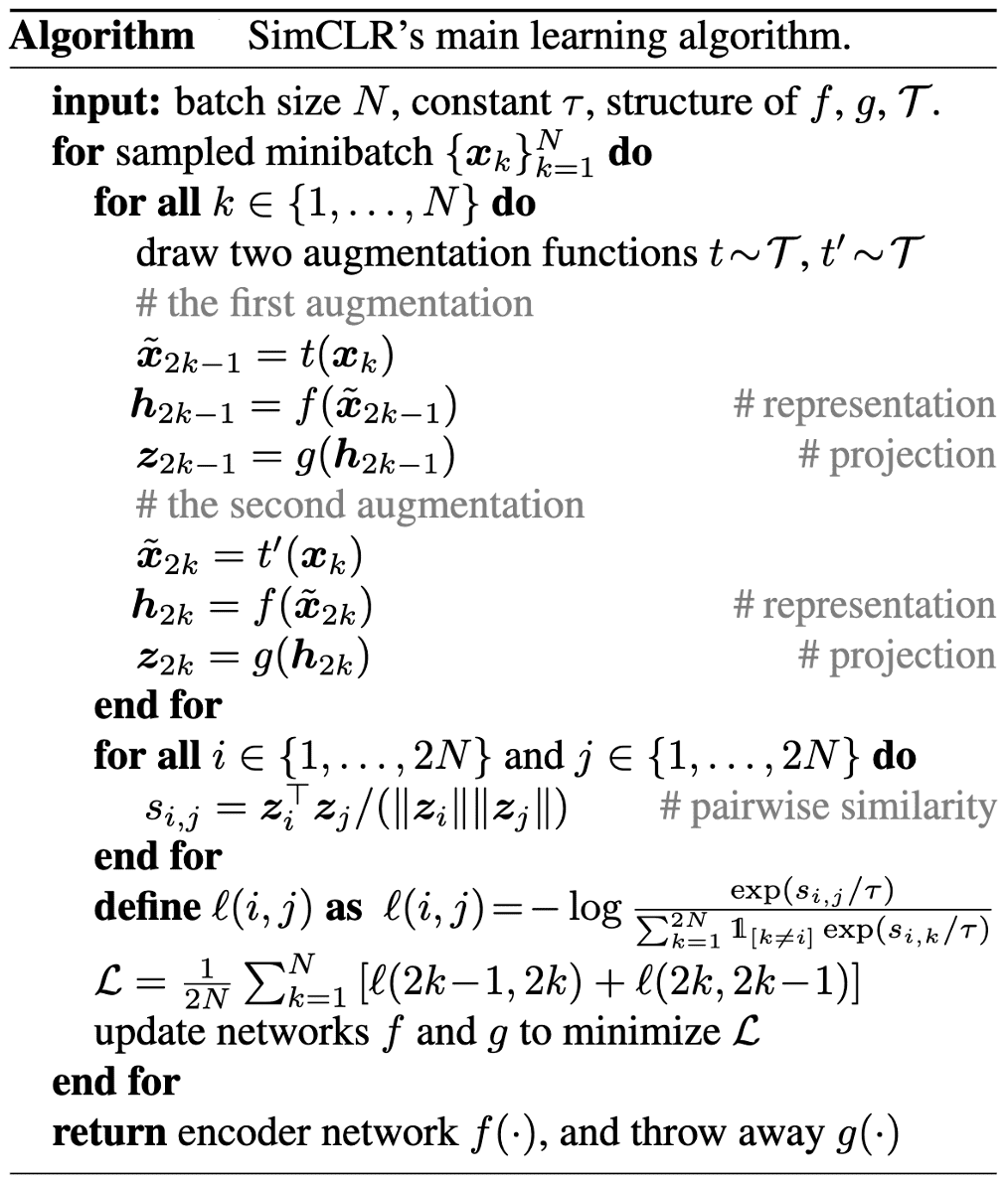
   Let $\text{sim}(\boldsymbol{u}, \boldsymbol{v}) = \boldsymbol{u}^\top \boldsymbol{v}/ \lVert \boldsymbol{u} \rVert \lVert \boldsymbol{v} \rVert$ be a cosine similarity. To identify $\tilde{\boldsymbol{x}}_j$ in $\{ \tilde{\boldsymbol{x}}_k \}_{k \neq i}$ for a given $\tilde{\boldsymbol{x}}_i$, the contrastive loss (termed NT-Xent) for a positive pair of examples $(i, j)$ is define as $$ \begin{aligned} \boldsymbol{z}_i &= g(\boldsymbol{h}_i) = W^{(2)} \text{ReLU}(W^{(1)} \boldsymbol{h}_i), \quad \boldsymbol{z}_j = g(\boldsymbol{h}_j) \\ \mathcal{L}^{(i,j)} &= - \log\frac{\exp(\text{sim}(\boldsymbol{z}_i, \boldsymbol{z}_j) / \tau)}{\sum_{k=1}^{2N} \mathbb{1}_{[k \neq i]} \exp(\text{sim}(\boldsymbol{z}_i, \boldsymbol{z}_k) / \tau)} \end{aligned} $$ where $\mathbb{1}_{[k \neq i]}$ is an indicator function and $\tau$ denotes a temperature parameter. A small neural network projection head $g(\cdot)$ that maps representations to the space where contrastive loss is applied. The authors find it beneficial to define the contrastive loss on $\boldsymbol{z}_i$’s rather than $\boldsymbol{h}_i$’s. Specifically, the mapping $\boldsymbol{z} = g(\boldsymbol{h})$ is trained to exhibit invariance to data transformations. Consequently, $g$ may eliminate information for the downstream task, such as the color or orientation of objects. Through the incorporation of $g(\cdot)$, a richer set of information can be constructed and preserved within $\boldsymbol{h}$.

$\mathbf{Fig\ 2.}$ The illustrated SimCLR framework (Ting Chen)

The following pseudocode outlines the overall training algorithm of SimCLR. The paper finds that the larger number of training epochs and batch sizes have a significant advantage, as it incorporates more negative example to the model.

$\mathbf{Fig\ 3.}$ SimCLR's training algorithm (Chen et al., 2020)

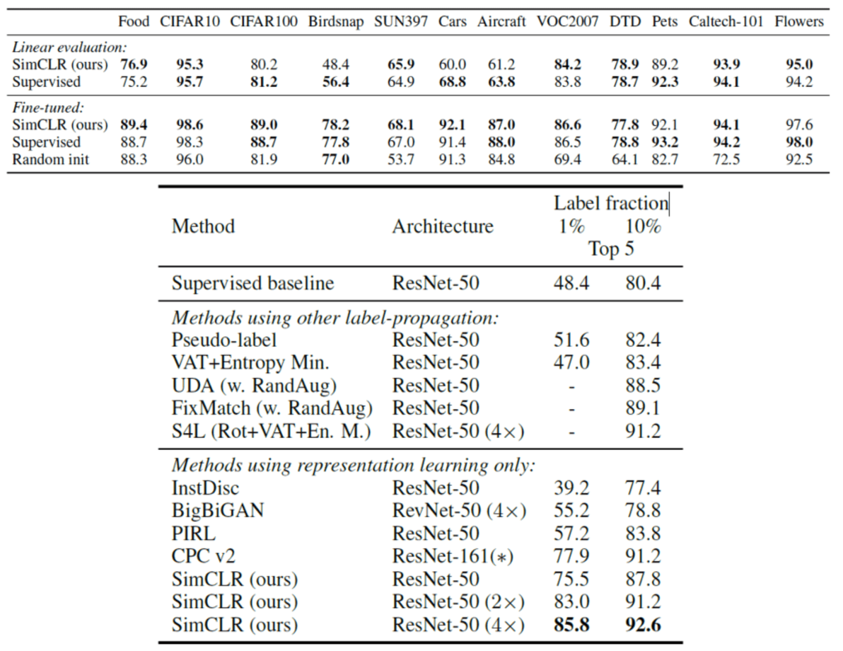
The paper evaluated the performance of SimCLR with

• linear evaluation
  • freeze the trained model and evaluate it by attaching a linear classifier on it
• fine-tuning
  • fine-tune both trained model and attached linear classifier
• transfer learning

As a consequence, SimCLR outperforms the previous self-supervised methods and approaches close to the performance of supervised model (trained on the dataset from scratch).

$\mathbf{Fig\ 4.}$ The performance of SimCLR (Chen et al., 2020)

SimCLR v2

Semi-supervised learning, learning from just a few labeled examples while making best use of a large amount of unlabeled data, remains a persistent challenge in the field of machine learning. Chen et al., NeurIPS 2020 developed an improved variant of SimCLR and proposed the new framework for semi-supervised learning termed SimCLRv2.

$\mathbf{Fig\ 5.}$ SimCLRv2 framework (Chen et al., NeurIPS 2020)

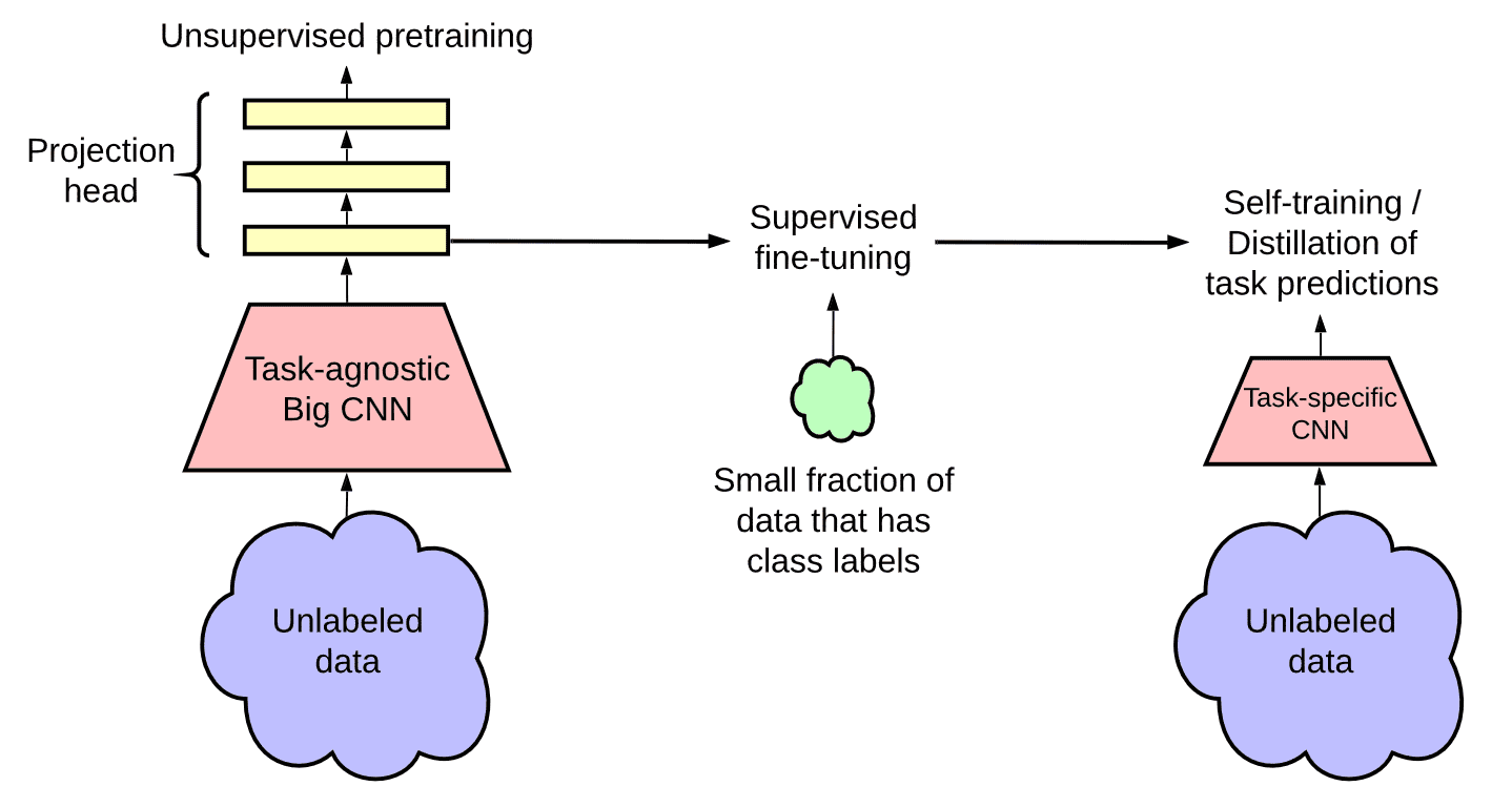
1. Unsupervised/Self-supervised pretraining
   The model leverages unlabeled data in task-agnostic way for learning general visual representations. It adopts the SimCLRv2, improved version of SimCLR in three major ways:
   1. Larger ResNet models for base encoder $f(\cdot)$; 152-layer ResNet with $3 \times$ wider channels and selective kernels
   2. Deeper projection head $g(\cdot)$; to increase the capacity to accomodate larger encoder
   3. Memory mechanism of MoCo
   
   Indeed, bigger encoders are more label-efficient for both supervised and semi-supervised learning, but gains appear to be larger for semi-supervised learning.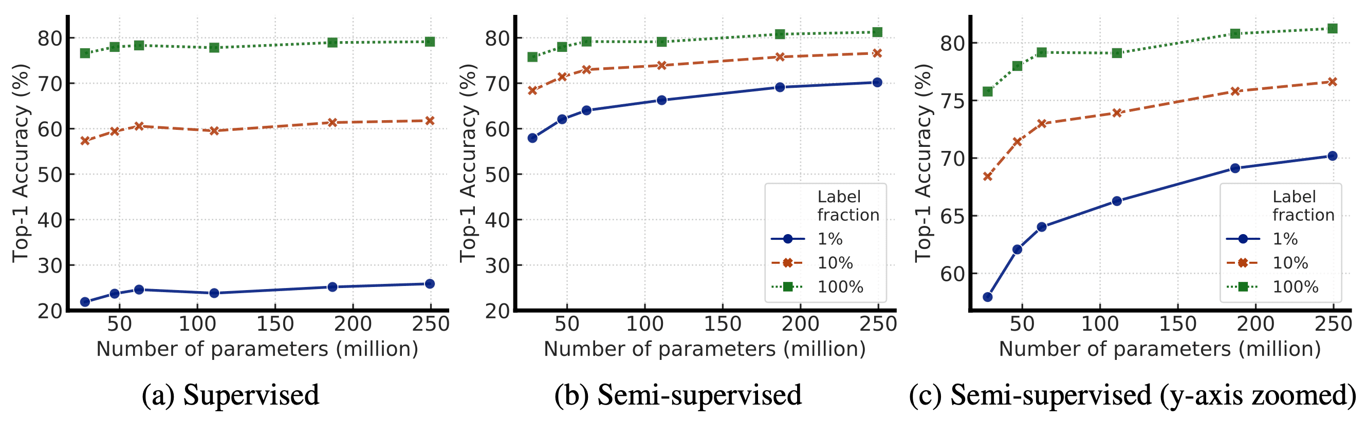

   

   $\mathbf{Fig\ 6.}$ Top-1 accuracy for supervised vs semi-supervised (SimCLRv2 fine-tuned) models of varied sizes (Chen et al., NeurIPS 2020)
   
   Although bigger models are better, some models can be more parameter efficient than others, hence searching for better architectures is always required.
2. Supervised fine-tuning
   Through fine-tuning, adapt the task-agnostically pretrained network for a specific task. In SimCLR, the MLP projection head $g(\cdot)$ is discarded entirely after pretraining, while only the ResNet encoder $f(\cdot)$ (the model from the input layer of the projection head) is used during the fine-tuning. Instead, SimCLR v2 incorporates part of the MLP projection head into the base encoder during the fine-tuning.
   
   Leveraging a deeper projection head during pre-training improves the performance when fine-tuning from the middle layer of projection head, and this middle layer is typically the first layer of projection head rather than the input (0th layer), especially with fewer labeled examples.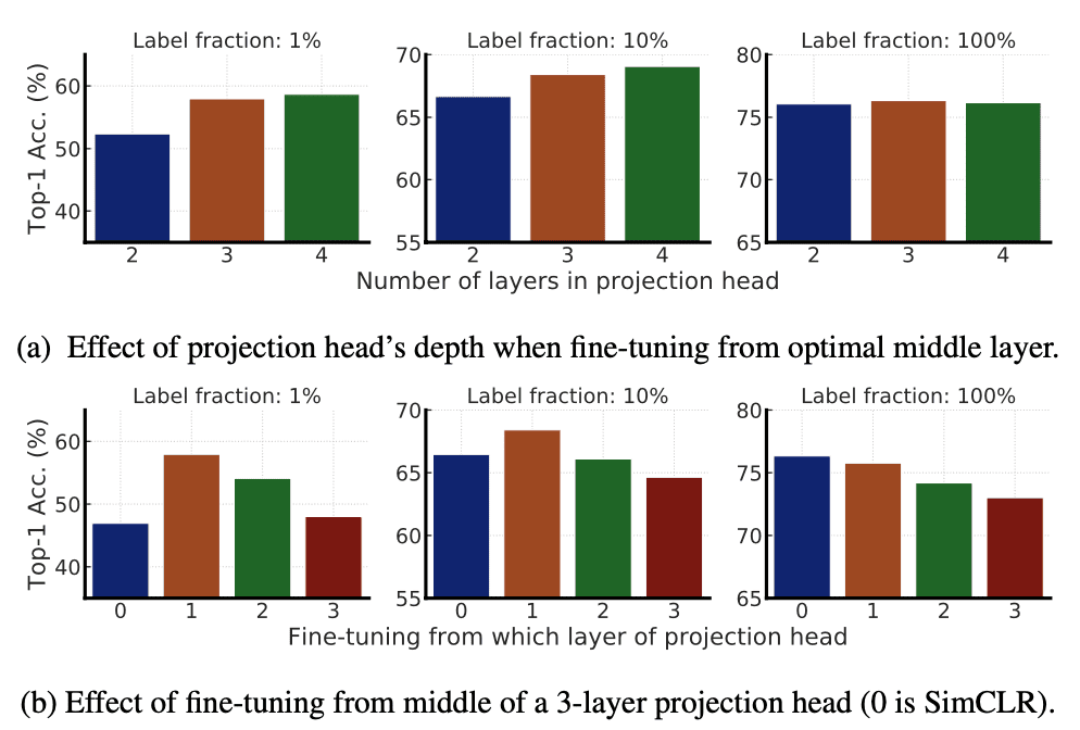

   

   $\mathbf{Fig\ 7.}$ Top-1 accuracy via fine-tuning under different projection head settings and label fractions (Chen et al., NeurIPS 2020)
   
   But increasing the depth of the projection head has limited effect when the projection head is already relatively wide. The improvement is larger with a smaller model size.
3. Self-training & Knowledge Distillation via Unlabeled Samples
   To further improve the network for the target task, SimCLR v2 leverages the unlabeled data directly for the target task. The fine-tuned network imputes the missing labels as a teacher for training a student network: $$ \mathcal{L}^{\text {distill }}=-\sum_{\boldsymbol{x}_i \in \mathcal{D}}\left[\sum_y P^T\left(y \mid \boldsymbol{x}_i ; \tau\right) \log P^S\left(y \mid \boldsymbol{x}_i ; \tau\right)\right] \text{ where } P(y \vert \boldsymbol{x}_i) = \frac{\exp f^{\text{task}} (\boldsymbol{x}_i) [y] / \tau}{\sum_{y^\prime} \exp f^{\text{task}} (\boldsymbol{x}_i) [y^\prime] / \tau} $$ Note that the teacher network that produces $P^T (y \vert \boldsymbol{x}_i)$ is fixed during the distillation; only the student network that produces $P^S (y \vert \boldsymbol{x}_i)$ is trained. The ground-truth labeled examples can be also combined with the distillation loss via a weighted combination when the number of labeled examples is sufficient: $$ \mathcal{L}=-(1-\alpha) \sum_{\left(\boldsymbol{x}_i, y_i\right) \in \mathcal{D}_{\text{labeled}}}\left[\log P^S\left(y_i \mid \boldsymbol{x}_i\right)\right]-\alpha \sum_{\boldsymbol{x}_i \in \mathcal{D}_{\text{unlabeled}}}\left[\sum_y P^T\left(y \mid \boldsymbol{x}_i ; \tau\right) \log P^S\left(y \mid \boldsymbol{x}_i ; \tau\right)\right] $$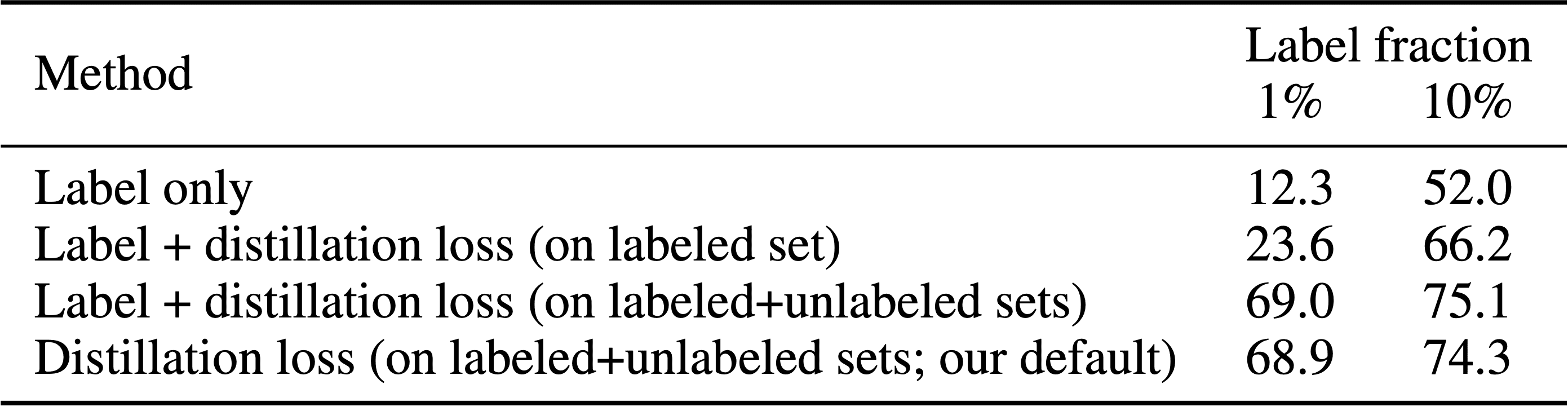

   

   $\mathbf{Fig\ 8.}$ Top-1 accuracy of a ResNet-50 trained on different types of losses. (Chen et al., NeurIPS 2020)
   
   
   Distillation with unlabeled examples improves fine-tuned models in two ways (See $\mathbf{Fig\ 9.}$):
   1. When the student model has a smaller architecture (in this case, the big model is self-distilled before distillation), it improves the model efficiency
   2. When the student model has the same architecture as the teacher model, it can still meaningfully improve the task-specific performance

   

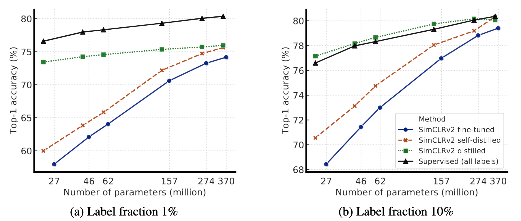
   $\mathbf{Fig\ 9.}$ Top-1 accuracy of distilled SimCLRv2 models.
   The self-distilled student has the same ResNet as the teacher (without MLP projection head)
   The distilled student is trained using the self-distilled ResNet-152
   (Chen et al., NeurIPS 2020)
   Note that self-distillation in this paper indicates the distillation when the teacher and the student have the same model architecture, not self-distillation of Zhang et al., 2019.

The following result shows the comparison of SimCLRv2 with previous state-of-the-art semi-supervised learning methods on ImageNet. SimCLRv2 significantly improves upon previous results, for both small and big ResNet variants, outperforming the state-of-the-art by a large margin.

$\mathbf{Fig\ 10.}$ ImageNet accuracy of models trained under semi-supervised settings (Chen et al., NeurIPS 2020)

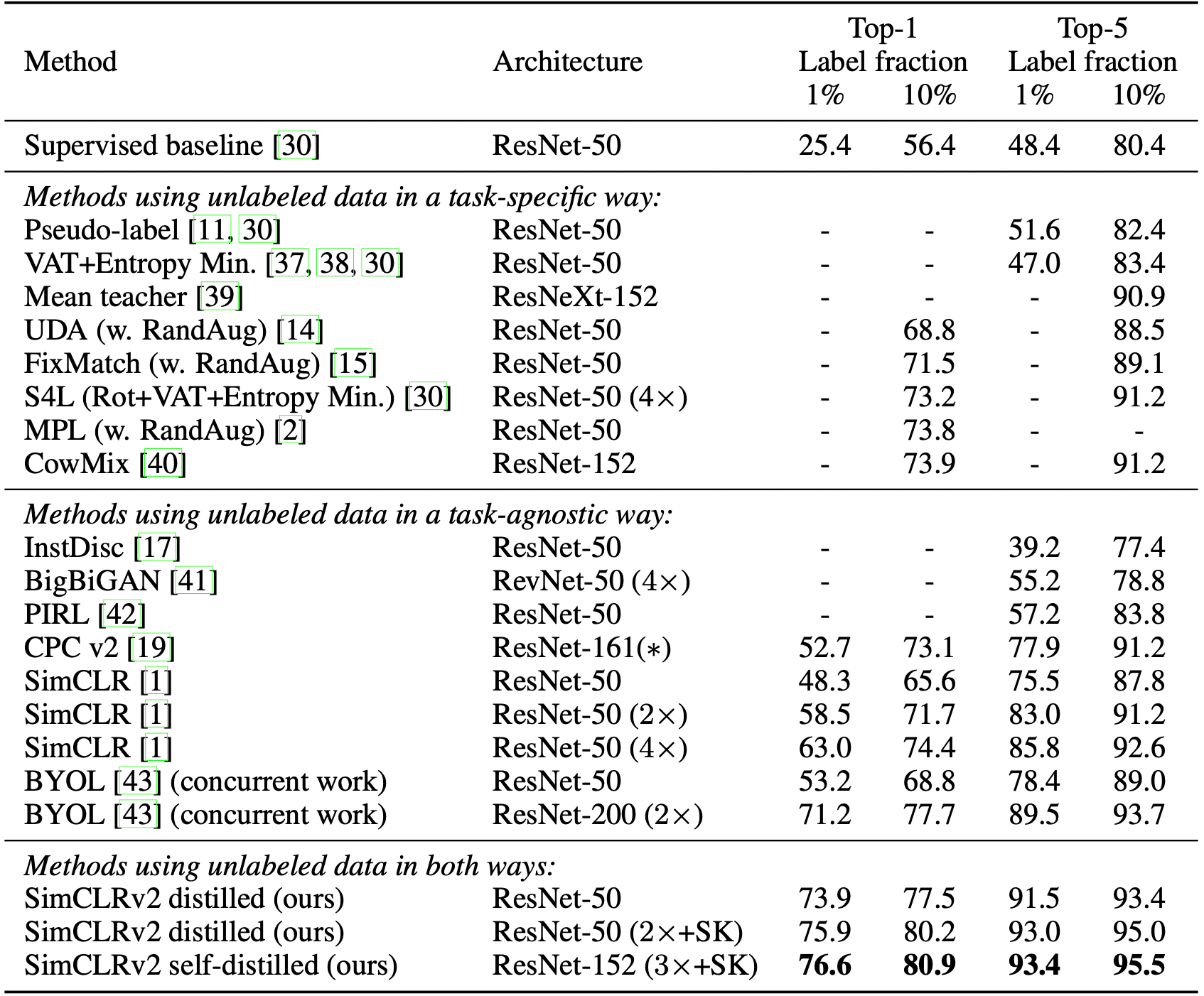
Nevertheless, it remains somewhat unexpected that larger models, susceptible to overfitting with limited labeled examples, exhibit superior generalization capabilities. By leveraging unlabeled data in a task-agnostic manner, the authors posit that larger models can acquire more generalized features, thereby enhancing the probability of learning task-relevant features. Nonetheless, they left further investigation as a future work to achieve a more comprehensive understanding of this phenomenon.

References

[1] Chen et al., “A Simple Framework for Contrastive Learning of Visual Representations.” International conference on machine learning. PMLR, 2020
[2] Amit Chaudhary, “The Illustrated SimCLR Framework”, 2020
[3] Ting Chen, “Advancing Self-Supervised and Semi-Supervised Learning with SimCLR”, Google Research Blog, 2020
[4] Chen et al., “Big Self-Supervised Models are Strong Semi-Supervised Learners” Advances in Neural Information Processing Systems. NeurIPS, 2020