[Representation Learning] Contrastive Multiview Coding (CMC)

The general approach in contrastive self-supervised learning for creating the positive views from a given image is to utilize two different random augmentations such as random crop, which generates views on the same dimension with the initial image.

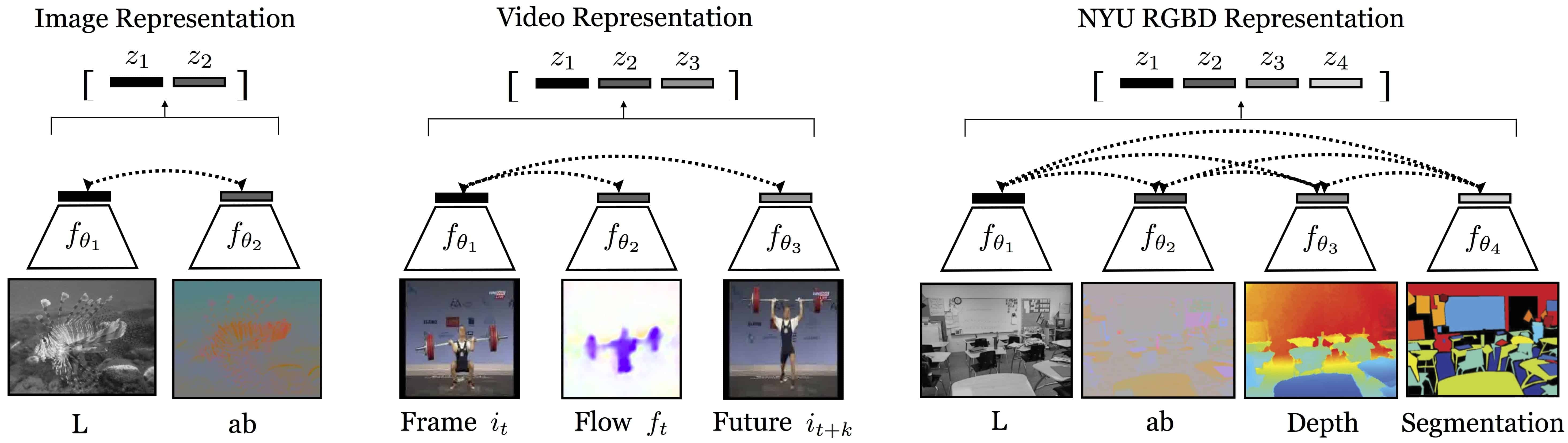
However, humans perceive the world through multiple sensory channels across different dimensions, such as luminance, chrominance, depth, and optical flow in the case of images. Building on this intuition, contrastive multiview coding (CMC) generates views by splitting an initial image into orthogonal dimensions, such as the luma and chroma dimensions. To achieve this, they extended the pairwise concept of contrastive learning to accommodate any number of views, which is the key contribution of the paper.

$\mathbf{Fig\ 1.}$ Contrastive Multiview Coding (Tian et al., ECCV 2020)

Multi-view Contrastive Learning

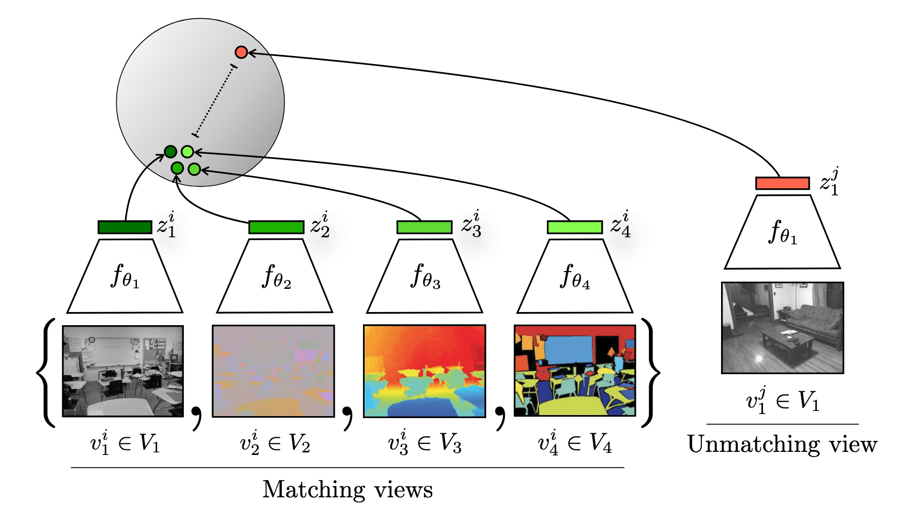
Consider a collection of $M$ views of the single data $\boldsymbol{x}$ across different channels, denoted as \(\mathbf{v}_1, \cdots, \mathbf{v}_M\). Using encoders \(f_{\theta_i}\) for each dimension $i = 1, \cdots, M$, these views are converted into representations $\mathbf{z}_1, \cdots, \mathbf{z}_M$:

\[\mathbf{z}_i = f_{\theta_i} (\mathbf{v}_i)\]

For brevity, denote $\bar{\mathbf{z}}_i$ the normalized feature $\mathbf{z}_i$, i.e., $\bar{\mathbf{z}}_i = \mathbf{z}_i / \Vert \mathbf{z}_i \Vert_2$.

Pairwise Contrastive Loss

Given a dataset of $V_1$ and $V_2$ that consists of a collection of positive pairs \(\{ \mathbf{v}_1^i, \mathbf{v}_2^i \}_{i=1}^N\), recall that the general pairwise contrastive loss is defined as follows:

\[\begin{gathered} \mathcal{L} (V_1, V_2) = \mathcal{L}_{\texttt{contrast}}^{V_1, V_2} + \mathcal{L}_{\texttt{contrast}}^{V_2, V_1} \\ \text{ where } \mathcal{L}_{\texttt{contrast}}^{V_1, V_2} = - \frac{1}{N} \sum_{i=1}^N \log \frac{\exp (\bar{\mathbf{z}}_1^i \cdot \bar{\mathbf{z}}_2^i / \tau)}{\sum_{j=1, j \neq i}^N \exp (\bar{\mathbf{z}}_1^i \cdot \bar{\mathbf{z}}_2^j / \tau)} \end{gathered}\]

Therefore, we may define the critic $h_\theta$ that consists of encoders $f_{\theta_1}$ and $f_{\theta_2}$ and outputs similarity scores between two views:

\[\begin{gathered} h_\theta (\mathbf{v}_1, \mathbf{v}_2) = \exp \left( \frac{f_{\theta_1} (\mathbf{v}_1)}{\Vert f_{\theta_1} (\mathbf{v}_1) \Vert_2} \cdot \frac{f_{\theta_2} (\mathbf{v}_2)}{\Vert f_{\theta_2} (\mathbf{v}_2) \Vert_2} \cdot \frac{1}{\tau} \right) \\ \Rightarrow \mathcal{L}_{\texttt{contrast}}^{V_1, V_2} = - \frac{1}{N} \sum_{i=1}^N \log \frac{h_\theta ( \mathbf{v}_1^i, \mathbf{v}_2^i )}{\sum_{j=1, j \neq i}^N h_\theta ( \mathbf{v}_1^i, \mathbf{v}_2^j )} \end{gathered}\]

Multi-view Contrastive Loss

Tian et al., 2020 presented multi-view formulation of contrastive loss using two paradigms:

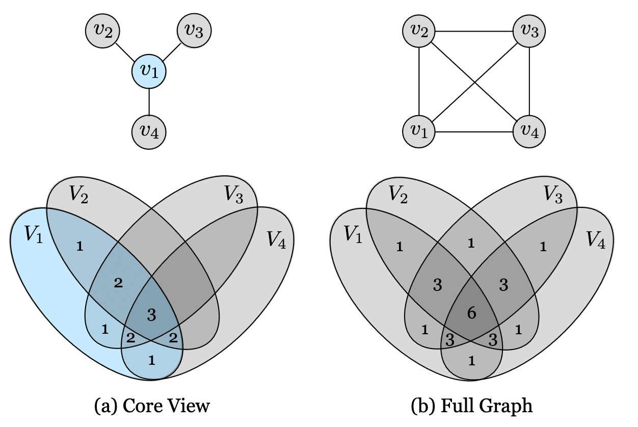
• Core view
  Set apart one view $V_1$ that we want to optimize over and build pair-wise loss with each other views $V_j (j > 1)$: $$ \mathcal{L}_C = \sum_{j=1}^M \mathcal{L}(V_1, V_j) $$
• Full graph
  Consider all $\binom{n}{2}$ combinations of pairs: $$ \mathcal{L}_F = \sum_{1 \leq i \leq j \leq M} \mathcal{L}(V_i, V_j) $$

$\mathbf{Fig\ 2.}$ Overview of CMC (Tian et al., ECCV 2020)

The information diagrams of two paradigms are visualized in the following figure. The numbers in the diagram indicate how many of the pairwise objectives that the partition contributes to. A factor that is common to more views, such as “presence of dog”, will be preferred over another factor that affects fewer views such as “depth sensor noise”.

$\mathbf{Fig\ 3.}$ The core view and full graph paradigms (Tian et al., ECCV 2020)

NCE Approximation

However, computing full softmax loss for each pair of the combination is not feasible with a large dataset such as ImageNet. Instead, the authors randomly sampled $m$ nagatives and performed $(m + 1)$-way softmax classification of noise-contrastive estimation (NCE) in Wu et al. 2018. The basic idea of NCE is to cast the multi-class classification into a set of binary classification problems.

Given an $i$-th example \(\mathbf{v}_1^i\) from $V_1$, the probability of \(\mathbf{v}_2\) from $V_2$ corresponds to the positive pair with \(\mathbf{v}_1^i\) was defined by critic $h_\theta$:

\[\mathrm{p}(\mathbf{v}_2 \vert \mathbf{v}_1^i) = \frac{h_\theta ( \mathbf{v}_1^i, \mathbf{v}_2 )}{\sum_{j=1}^N h_\theta ( \mathbf{v}_1^i, \mathbf{v}_2^j )}\]

Since the normalization factor (denominator) is expensive for large $N$, NCE instead formulates a binary classfier $\mathbb{P}$ to estimate $\mathrm{p}$:

\[\mathrm{p}(\mathbf{v}_2 \vert \mathbf{v}_1^i) = \mathbb{P}(D = 1 \vert \mathbf{v}_2; \mathbf{v}_1^i)\]

where $\mathbb{P}$ distinguishes the positive sample $\mathbf{v}_2^i$ from $m$ noise (negative) samples of the distribution $\mathrm{p}_n (\cdot \vert \mathbf{v}_1^i)$

\[\mathbb{P} (D = 1 \vert \mathbf{v}_2; \mathbf{v}_1^i) = \frac{\mathrm{p}_d (\mathbf{v}_2 \vert \mathbf{v}_1^i)}{\mathrm{p}_d (\mathbf{v}_2 \vert \mathbf{v}_1^i) + m \mathrm{p}_n (\mathbf{v}_2 \vert \mathbf{v}_1^i)}\]

Here, \(\mathrm{p}_d (\cdot \vert \mathbf{v}_1^i)\) is an unknown distribution that we need to estimate. Hence, the authors modeled \(\mathrm{p}_d (\mathbf{v}_2 \vert \mathbf{v}_1^i)\) with \(h_\theta (\mathbf{v}_1^i, \mathbf{v}_2) / Z_0\) where $Z_0$ is a constant and set $\mathrm{p}_n = \frac{1}{N}$. The final objective is therefore modified using the following approximation of pair-wise contrastive loss:

\[\mathcal{L}_{\texttt{contrast}}^{V_1, V_2} \approx \mathcal{L}_{\texttt{NCE}} = - \frac{1}{N} \sum_{i=1}^N \left[ \log \mathbb{P}(D = 1 \vert \mathbf{v}_2^i; \mathbf{v}_1^i) + \sum_{j=1}^m \log \mathbb{P}(D = 0 \vert \mathbf{v}_2^{n_j}; \mathbf{v}_1^i) \right]\]

where $n_j$ are sampled indices for negative samples, i.e., \(n_j \in \{ 1, \cdots, N \} - i\).

Properties

To explore the properties of CMC, the authors experimented on the NYU-Depth-V2 dataset that consists of the 5 channels: luminance ($L$), chrominance ($ab$), depth, surface normal, and semantic labels.

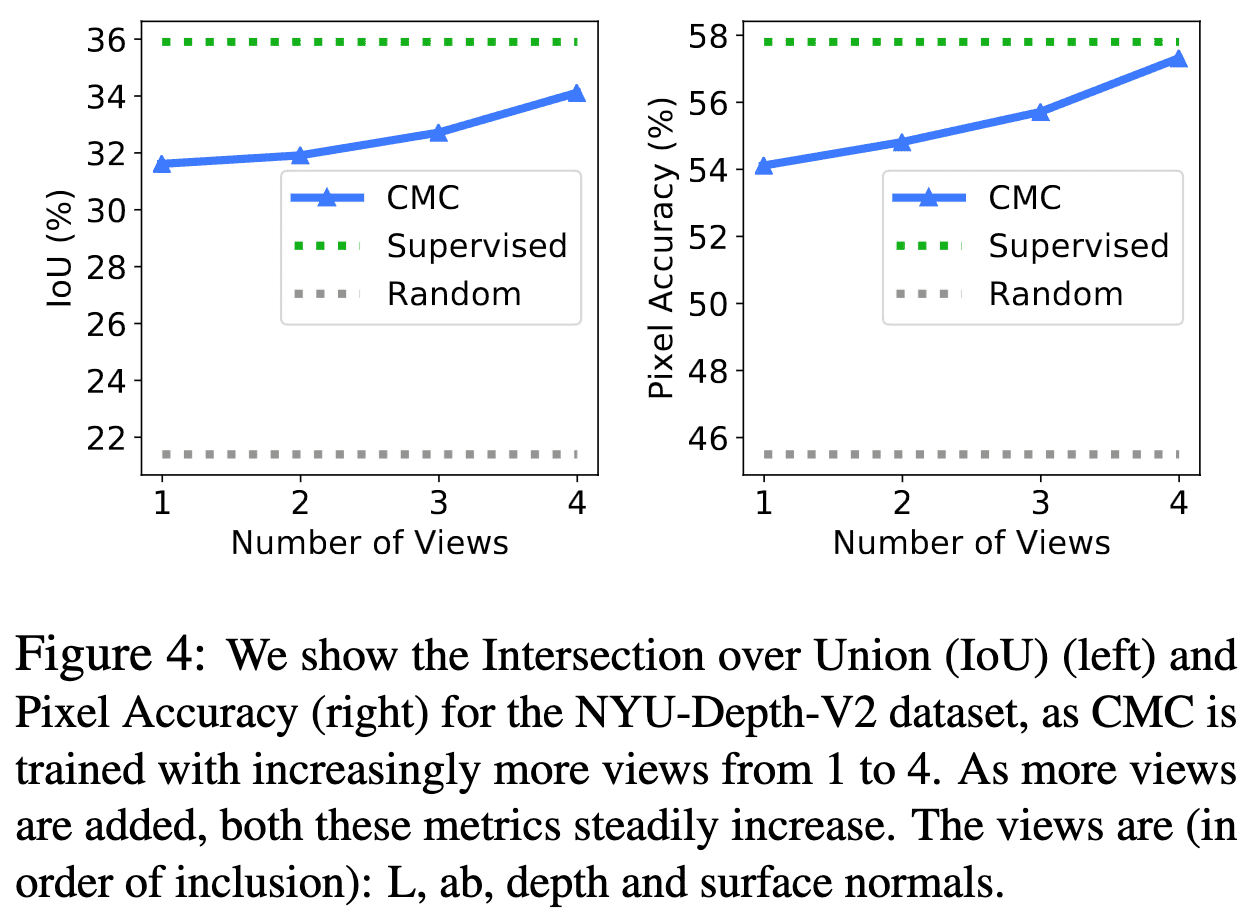
The More Views, The Better Performance

To measure the quality of the learned representation, they considered core view paradigm for predicting semantic labels from the representation of $L$ as the core view. As a result, as the number of views increases (regardless of the order of adding views), the accuracy of CMC steadily improves.

$\mathbf{Fig\ 4.}$ As more views are added, both these metrics steadily increase. (Tian et al., ECCV 2020)

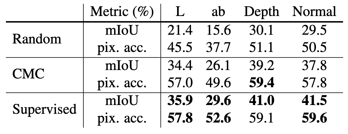
CMC Improves All Views

To investigate that CMC improve the quality of representations for all views, they considered the full graph paradigm for predicting the semantic labels from a single view $v$, where $v$ can be $L$, $ab$, depth, or surface normal. The authors observed that CMC framework improves the quality of unsupervised representations, bringing them closer to the quality of supervised ones across all views investigated.

$\mathbf{Fig\ 5.}$ Performance on the task of using single view $v$ to predict the semantic labels. (Tian et al., ECCV 2020)

References

[1] Tian et al., “Contrastive Multiview Coding”, ECCV 2020
[2] Wu et al., “Unsupervised Feature Learning via Non-Parametric Instance-level Discrimination”, CVPR 2018
[3] Official Implementation of CMC