[Representation Learning] Supervised Contrastive Learning (SupCon)

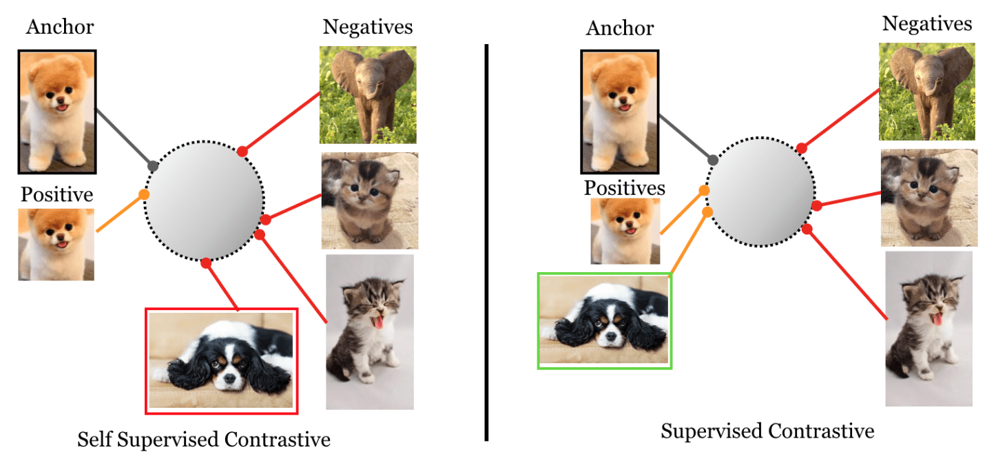
Contrastive learning framework for self-supervised representation learning has shown superior performances in recent years, leading to state of the art performance in the unsupervised training of deep vision models. To construct contrastive loss, for instance, SimCLR creates positive pairs by applying two different random augmentations $\mathcal{T}$ and $\mathcal{T}^\prime$ to an initial image $\boldsymbol{x}$ twice.

If we can access to additional information, such as categorical labels, we may use this framework to select positive pairs with the same label, and negative pairs with different labels. With this simple intuition, Khosla et al., 2020 extended the self-supervised contrastive approach to the fully-supervised setting, allowing us to effectively leverage label information.

$\mathbf{Fig\ 1.}$ Supervised vs. self-supervised contrastive losses (Khosla et al., 2020)

The resulting objective with a contrastive loss is called Supervised Contrastive Loss (SupCon), and resembles neighborhood component analysis. It has been shown to improve robustness compared to standard supervised learning losses.

Supervised Contrastive Losses

Suppose that a batch of $N$ randomly samples sample/label pairs \(\{ \boldsymbol{x}_k, y_k \}_{k=1}^N\) is given. As usual contrastive learning framework, generate the multi-viewed batch consists of $2N$ pairs \(\{ \tilde{\boldsymbol{x}}_\ell, \tilde{y}_\ell \}_{\ell=1}^{2N}\) using two different random augmentations $\mathcal{T}_1$, $\mathcal{T}_2$ where

\[\begin{aligned} \tilde{\boldsymbol{x}}_{2k - 1} & = \mathcal{T}_1 (\boldsymbol{x}_k) \\ \tilde{\boldsymbol{x}}_{2k} & = \mathcal{T}_2 (\boldsymbol{x}_k) \\ \tilde{y}_{2k - 1} & = \tilde{y}_{2k} = y_k \end{aligned}\]

Then, similar to SimCLR, these different views are processed by the base encoder $f$ followed by the projection head $h$: \(\boldsymbol{z}_\ell = g(f(\boldsymbol{x}_{\ell}))\). For index set \(\mathcal{I} = \{ 1, \cdots, 2N \}\), let denote $\mathcal{P} (\ell) \subseteq \mathcal{I}$ the index set of positive pairs of $\ell \in \mathcal{I}$.

Self-Supervised Contrastive Loss

Recall that self-supervised contrastive loss is defined by:

\[\mathcal{L}^{\texttt{self-sup}} = - \sum_{\ell \in \mathcal{I}} \log \frac{\exp (\boldsymbol{z}_\ell \cdot \boldsymbol{z}_{ \mathcal{P}(\ell) } / \tau) }{\sum_{i \in \mathcal{I} - \ell} \exp (\boldsymbol{z}_\ell \cdot \boldsymbol{z}_i / \tau)}\]

where

\[\mathcal{P}(\ell) = \begin{cases} 2k & \quad \text{ if } \ell = 2k-1 \text{ for some } k = 1, \cdots, N \\ 2k - 1 & \quad \text{ if } \ell = 2k \text{ for some } k = 1, \cdots, N \\ \end{cases}\]

Supervised Contrastive Losses

Now, in fully-supervised setting, the set of indices of all positives in the multi-viewed batch of $\ell$-th feature can be defined by:

\[\mathcal{P} (\ell) = \{ p \in \mathcal{I} - \ell \vert \tilde{y}_p = \tilde{y}_i \}\]

The following two losses are most straightforward, depending on the location of $\log$, to generalize $\mathcal{L}^{\texttt{self-sup}}$ to an arbitary number of positives:

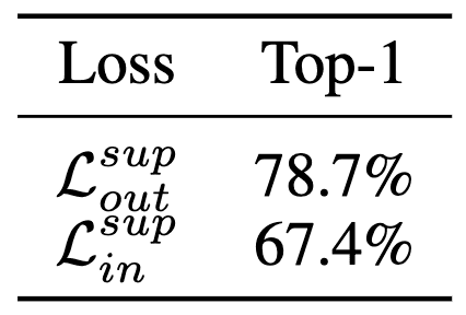
\[\begin{aligned} \mathcal{L}_{\texttt{out}}^{\texttt{sup}} & = - \sum_{\ell \in \mathcal{I}} \frac{1}{\vert \mathcal{P}(\ell) \vert} \sum_{p \in \mathcal{P}(\ell)} \log \frac{\exp (\boldsymbol{z}_\ell \cdot \boldsymbol{z}_p / \tau)}{\sum_{i \in \mathcal{I} - \ell} \exp (\boldsymbol{z}_\ell \cdot \boldsymbol{z}_i / \tau) } \\ \mathcal{L}_{\texttt{in}}^{\texttt{sup}} & = - \sum_{\ell \in \mathcal{I}} \log \left\{ \frac{1}{\vert \mathcal{P}(\ell) \vert} \sum_{p \in \mathcal{P}(\ell)} \frac{\exp (\boldsymbol{z}_\ell \cdot \boldsymbol{z}_p / \tau)}{\sum_{i \in \mathcal{I} - \ell} \exp (\boldsymbol{z}_\ell \cdot \boldsymbol{z}_i / \tau) } \right\} \end{aligned}\]

Note that \(\mathcal{L}_{\texttt{in}}^{\texttt{sup}} \leq \mathcal{L}_{\texttt{out}}^{\texttt{sup}}\) by Jensen’s inequality. Since \(\mathcal{L}_{\texttt{out}}^{\texttt{sup}}\) is an upper bound of \(\mathcal{L}_{\texttt{in}}^{\texttt{sup}}\), we can deduce that \(\mathcal{L}_{\texttt{out}}^{\texttt{sup}}\) is more advantageous to the performance.

$\mathbf{Fig\ 2.}$ ImageNet Top-1 classification accuracy for supervised contrastive losses (Khosla et al., 2020)

Therefore, the supervised contrastive (SupCon) loss is defined by:

\[\begin{gathered} \mathcal{L}^{\texttt{sup}} = - \sum_{\ell \in \mathcal{I}} \frac{1}{\vert \mathcal{P}(\ell) \vert} \sum_{p \in \mathcal{P}(\ell)} \log \frac{\exp (\boldsymbol{z}_\ell \cdot \boldsymbol{z}_p / \tau)}{\sum_{i \in \mathcal{I} - \ell} \exp (\boldsymbol{z}_\ell \cdot \boldsymbol{z}_i / \tau) } \\ \text{ where } \mathcal{P} (\ell) = \{ p \in \mathcal{I} - \ell \vert \tilde{y}_p = \tilde{y}_i \} \end{gathered}\]

Gradient Analysis

Furthermore, the following gradient analysis of two losses suggests that the positives normalization factor $1 / \vert \mathcal{P} (\ell) \vert$ contributes to remove bias present within the positive sets in a multi-viewed batch.

Observe that the gradient for either \(\mathcal{L}_{\texttt{in}, \ell}^{\texttt{sup}}\) or \(\mathcal{L}_{\texttt{out}, \ell}^{\texttt{sup}}\) has the following form:

\[\begin{aligned} \frac{\partial \mathcal{L_{\ell}^\texttt{sup}}}{\partial \boldsymbol{z}_\ell} = \frac{1}{\tau} \left\{ \sum_{p \in \mathcal{P}(\ell)} \boldsymbol{z}_p (P_{\ell p} - X_{\ell p}) + \sum_{n \in \mathcal{N}(\ell)} \boldsymbol{z}_n P_{\ell n} \right\} \end{aligned}\]

where \(\mathcal{N}(\ell) = \{ n \in \mathcal{I} - \ell \vert n \notin \mathcal{P}(\ell) \}\) is the index set of all negatives and

\[\begin{aligned} P_{\ell j} & = \frac{\exp (\boldsymbol{z}_\ell \cdot \boldsymbol{j} / \tau)}{\sum_{i \in \mathcal{I} - \ell} \exp (\boldsymbol{z}_\ell \cdot \boldsymbol{i} / \tau)} \\ X_{\ell p} & = \begin{cases} \frac{\exp (\boldsymbol{z}_\ell \cdot \boldsymbol{z}_p / \tau)}{\sum_{p^\prime \in \mathcal{P}(\ell)} \exp (\boldsymbol{z}_\ell \cdot \boldsymbol{z}_{p^\prime} / \tau)} & \quad \text{ if } \mathcal{L}_{\ell}^{\texttt{sup}} = \mathcal{L}_{\texttt{in}, \ell}^{\texttt{sup}}\\ \frac{1}{\vert \mathcal{P}(\ell) \vert} & \quad \text{ if } \mathcal{L}_{\ell}^{\texttt{sup}} = \mathcal{L}_{\texttt{out}, \ell}^{\texttt{sup}} \end{cases} \end{aligned}\]

If each \(\boldsymbol{z}_p\) is set to the mean positive representation vector \(\bar{\boldsymbol{z}}\), which is less biased, \(X_{\ell p}^{\texttt{in}}\) reduces to \(X_{\ell p}^{\texttt{out}}\):

\[\left. X_{\ell p}^{\texttt{in}}\right|_{\boldsymbol{z}_p = \bar{\boldsymbol{z}}} = \frac{\exp (\boldsymbol{z}_\ell \cdot \bar{\boldsymbol{z}} / \tau)}{\sum_{p^\prime \in \mathcal{P}(\ell)} \exp (\boldsymbol{z}_\ell \cdot \bar{z} / \tau )} = \frac{\exp (\boldsymbol{z}_\ell \cdot \bar{\boldsymbol{z}} / \tau)}{\vert \mathcal{P} (\ell) \vert \cdot \exp (\boldsymbol{z}_\ell \cdot \bar{z} / \tau)} = \frac{1}{\vert \mathcal{P}(\ell) \vert}=X_{\ell p}^{\texttt {out}}\]

Therefore, \(\mathcal{L}_{\texttt{out}}^{\texttt{sup}}\) can be considered as the stabilized form of \(\mathcal{L}_{\texttt{in}}^{\texttt{sup}}\) by using the mean of positives. Since the normalization factor $1 / \vert \mathcal{P} (\ell) \vert$ is located inside of the $\log$ in case of $\mathcal{L}_{\texttt{in}}^{\texttt{sup}}$, it thus contributes only an additive constant to the overall loss, which does not affect the gradient, and is more susceptible to bias in the positives.

Experimental Results

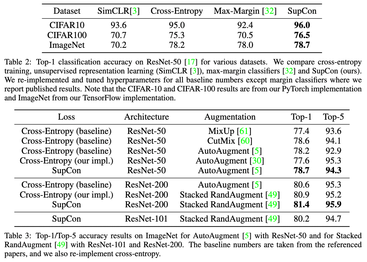
As a result, SupCon generalizes better than cross-entropy, margin classifiers (with labels) and unsupervised contrastive learning techniques in classification tasks on CIFAR-10, CIFAR-100 and ImageNet datasets. Especially, it consistently outperforms cross-entropy loss with standard data augmentations, demonstrating a new state-of-the-art accuracy.

$\mathbf{Fig\ 3.}$ Classification accuracy results (Khosla et al., 2020)

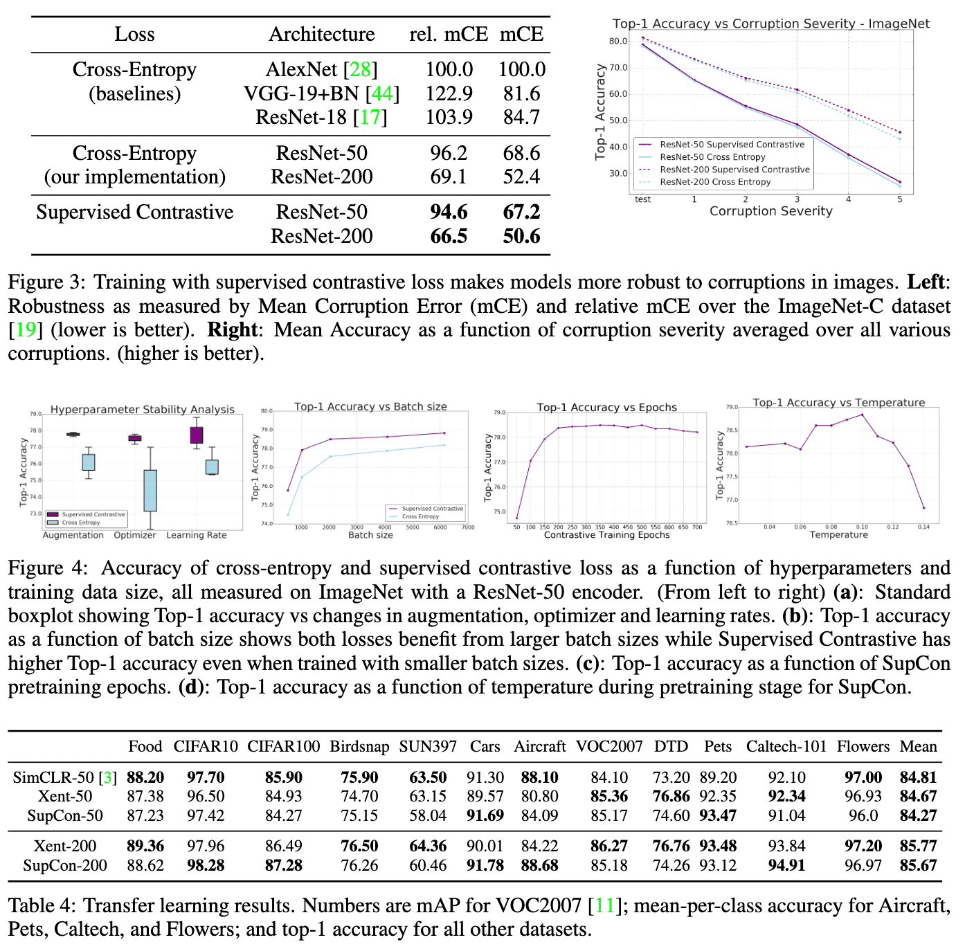
In general, vision models exhibit a lack of robustness to out-of-distribution data or natural corruptions such as noise, blur and JPEG compression. When comparing the SupCon models to cross-entropy on ImageNet-C benchmark, SupCon has shown less degradation in accuracy with increasing corruption severity, which suggests for increased robustness. Furthermore, SupCon was more robust to the choice of hyperparameters such as batch sizes and augmentation.

$\mathbf{Fig\ 4.}$ Robustness of SupCon (Khosla et al., 2020)

Reference

[1] Khosla et al., “Supervised Contrastive Learning”, NeurIPS 2020