
[Representation Learning] BYOL
Introduction
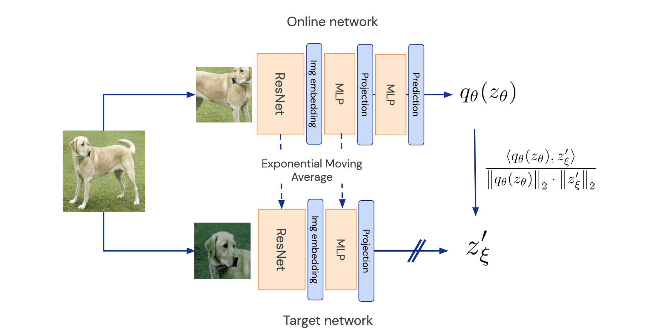
Various contrastive learning-based methods for learning image representations leverage the positive pairs and negative pairs, which require the careful treatement to retrieve the large amount of negative pairs, e.g. memory banks in MoCo, batch size in SimCLR. Bootstrap Your Own Latent (BYOL, Grill et al. NeurIPS 2020) is an algorithm for self-supervised learning of image representations without using negative pairs that directly bootstrap the representations. To do so, BYOL uses two neural networks, referred to as online and target networks, that interact and learn from each other. In particular, the target network yields the target representation with different view of an image and the online network is tasked to predict the target representation produced by the target network so as to train a new, potentially enhanced and generalized representation.
The core motivation for BYOL is the following experimental finding. The authors found that bootstrapping the representation has potential to significantly enhance the quality of learned representation: While a fixed randomly initialized network only achieves 1.4% top-1 accuracy on the linear evaluation on ImageNet, the network trained to predict the targets produced by the fixed randomly initialized network achieves 18.8% top-1 accuracy. Therefore, by iterating this procedure and using subsequent online networks as new target networks for further training, we can anticipate constructing a sequence of representations of increasing quality. And BYOL generalizes this bootstrapping procedure by iteratively refining its representation but utilizes a slowly moving exponential average of the online network as the target network instead of employing fixed checkpoints.
BYOL
The online network is parameterized by a set of weights $\theta$ and comprised of three modules:
- encoder $f_\theta$
- projector $g_\theta$
- predictor $q_\theta$
The target network has the same architecture as the online network (but uses a different set of weights $\xi$) provides the regression targets to train the online network. It is updated by an exponential moving average $\xi \leftarrow \tau \xi + (1 - \tau) \theta$ with $\tau \in [0, 1]$ after each training step. Then, BYOL operates as follows:
- Create different views of single image
Given a set of images $\mathcal{D}$, an image $\mathbf{x} \sim \mathcal{D}$ sampled uniformly, and two distributions of image augmentations $\mathcal{T}$ and $\mathcal{T}^\prime$, BYOL produces two augmented views $\mathbf{v} = t(\mathbf{x})$ and $\mathbf{v}^\prime = t^\prime(\mathbf{x})$ from sampled augmentations $t \sim \mathcal{T}$ and $t^\prime \sim \mathcal{T}^\prime$. - Obtain representation $\mathbf{y}$ and projection $\mathbf{z}$
Obtain representation $\mathbf{y}_{\theta}$ and projection $\mathbf{z}_\theta$ for the first view $\mathbf{v}$ from the online network: $$ \begin{aligned} \mathbf{y}_\theta & = f_\theta (\mathbf{v}) \\ \mathbf{z}_\theta & = g_\theta ( \mathbf{y}_\theta ) \end{aligned} $$ And for $\mathbf{v}^\prime$ from the target network: $$ \begin{aligned} \mathbf{y}^\prime_\xi & = f_\xi (\mathbf{v}^\prime ) \\ \mathbf{z}^\prime_\xi & = g_\xi ( \mathbf{y}^\prime_\xi ) \end{aligned} $$ - Prediction and $\ell_2$ normalization
The online network outputs a prediction $q_\theta (\mathbf{z}_\theta)$ of $\mathbf{z}^\prime_\xi$ and $\ell_2$-normalize them $$ \bar{q_\theta}(\mathbf{z}_\theta) = \frac{q_\theta(\mathbf{z}_\theta)} {\lVert q_\theta(\mathbf{z}_\theta) \rVert_2}, \quad \bar{\mathbf{z}}^\prime_\xi = \frac{\mathbf{z}^\prime_\xi} {\lVert \mathbf{z}^\prime_\xi \rVert_2} $$ Note that this predictor is only applied to the online branch, making the architecture asymmetric between the online and target network pipeline. - Calculate MSE loss between the normalized predictions and target projections
$$ \mathcal{L}_{\theta, \xi} = \lVert \bar{q_\theta}(\mathbf{z}_\theta) - \bar{\mathbf{z}}^\prime_\xi \rVert_2^2 = 2 - 2 \times \frac{\left< q_\theta(\mathbf{z}_\theta), \mathbf{z}^\prime_\xi \right>}{\lVert q_\theta(\mathbf{z}_\theta) \rVert_2 \cdot \lVert \mathbf{z}^\prime_\xi \rVert_2} $$ - Symmetrize the loss by switching $\mathbf{v}^\prime$ and $\mathbf{v}$, obtaining $\tilde{\mathcal{L}}_{\theta, \xi}$
$$ \mathcal{L}^{\textrm{BYOL}}_{\theta, \xi} = \mathcal{L}_{\theta, \xi} + \tilde{\mathcal{L}}_{\theta, \xi} $$ - Parameter optimization
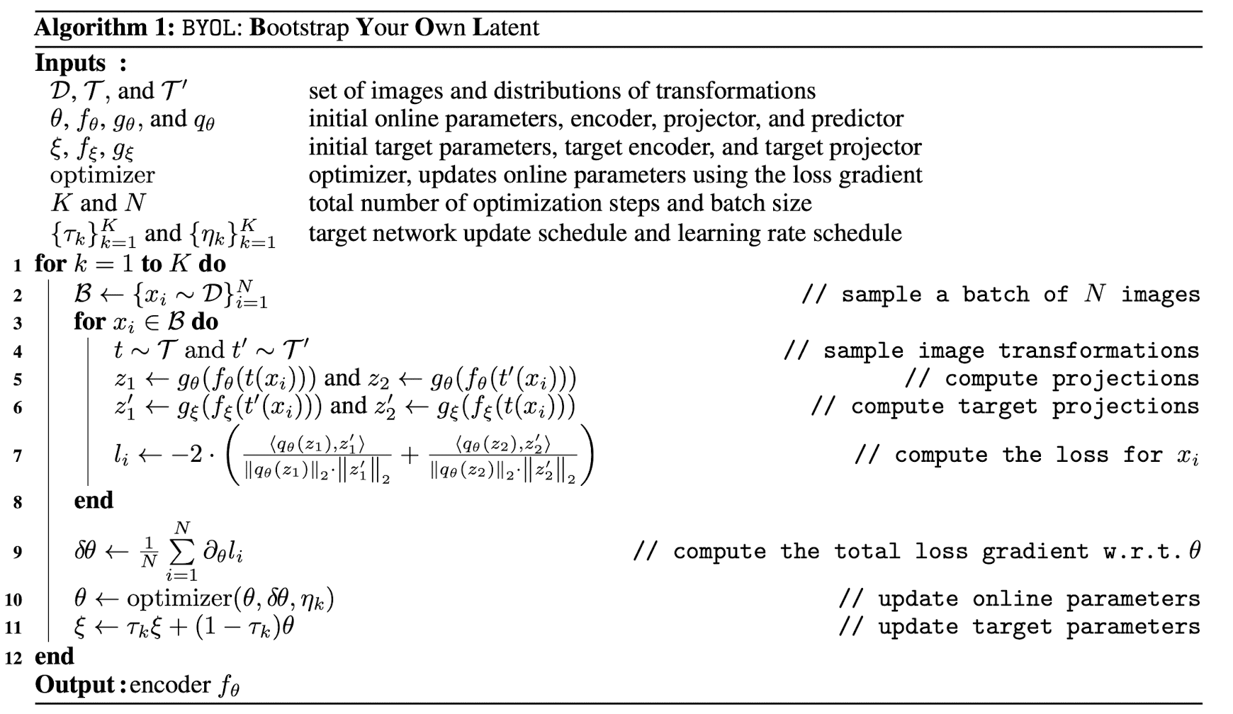
$$ \begin{aligned} & \theta \leftarrow \operatorname{optimizer}\left(\theta, \nabla_\theta \mathcal{L}_{\theta, \xi}^{\mathrm{BYOL}}, \eta\right) \\ & \xi \leftarrow \tau \xi+(1-\tau) \theta \end{aligned} $$ where $\operatorname{optimizer}$ is an optimizer and $\eta$ is a learning rate. In practice, the exponential moving average parameter $\tau$ starts from $\tau_{\textrm{base}} = 0.996$ and is increased to $1$ during training by cosine annealing: $\tau = 1 - (1 - \tau_{\textrm{base}}) \cdot (\cos (\pi k / K) + 1) / 2$.
$\mathbf{Fig\ 2}$ shows the whole algorithm of BYOL training algorithm.
Experiment Results
Representation Evaluation
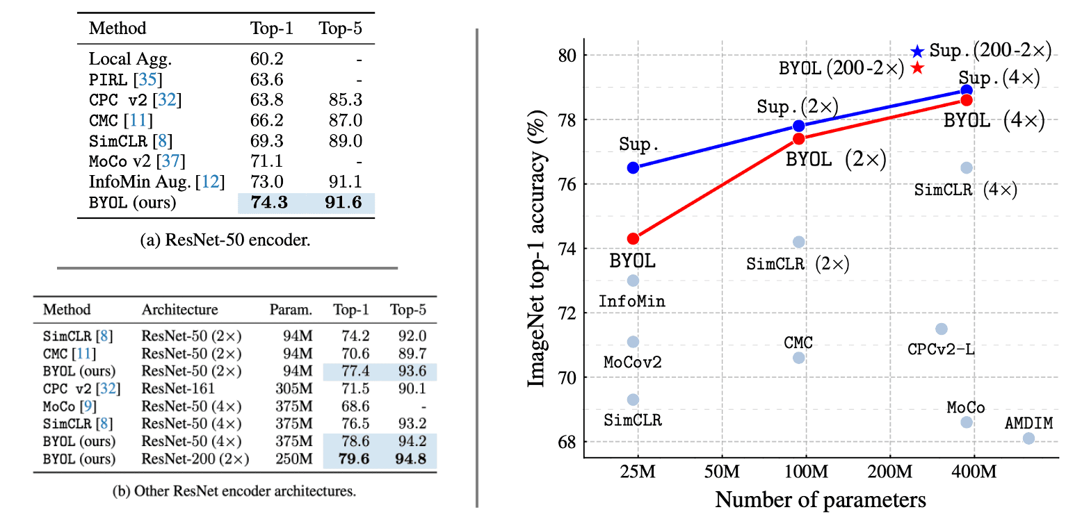
Under the linear evaluation protocol on ImageNet, consisting in training a linear classifier on top of the frozen representation, BYOL reaches 74.3% top-1 accuracy with a standard ResNet-50 and 79.6% top-1 accuracy with a larger ResNet, ranking higher than previous self-supervised approaches.
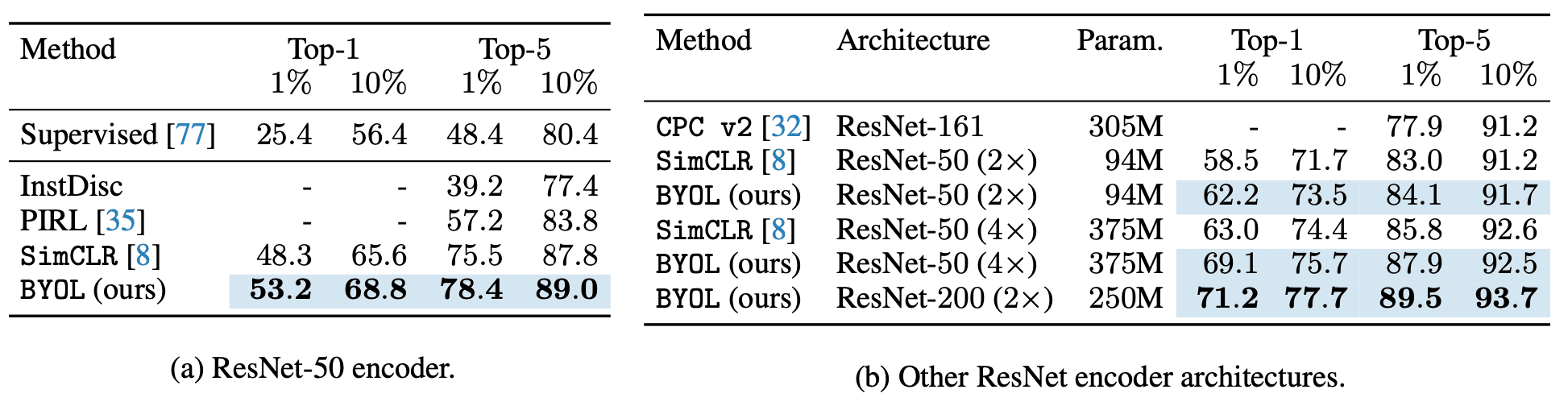
Next, the paper evaluates the performance obtained when fine-tuning BYOL’s representation on classification task with a small subset of ImageNet’s train set with label information. As a result, BYOL exhibits results on par or superior to the previous state-of-the-art.
Ablation Study
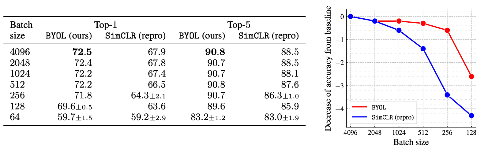
Since BYOL does not use negative examples, it is more robust to smaller batch sizes as the following ablation study exhibits. Although the performance of SimCLR rapidly deteriorates with batch size, likely due to the decrease in the number of negative examples, BYOL remains stable over a wide range of batch sizes from 256 to 4096.
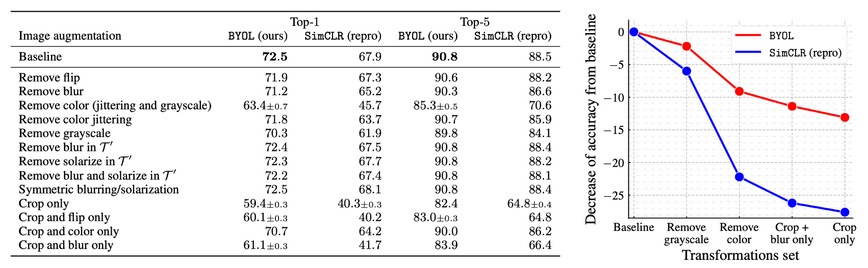
Moreover, contrastive methods such as SimCLR are usually sensitive to the combinations of image augmentations. For instance, while crops of the same image mostly share their color histograms, color histograms vary across images. Therefore, relying only on random crops as augmentations, it can be mostly solved by focusing on color histograms alone, discouraging the representation from retaining broader information. To prevent that, SimCLR should add color distortion to its set of transformations. Instead, BYOL is motivated to retain any information present in the target representation within its online network to enhance predictions. Consequently, BYOL will exhibit greater robustness to the selection of image augmentations, and the following experiment supports the hypothesis.
Avoiding collapsed representations
Many successful self-supervised learning approaches learn representations by predicting the representation of differently augmented views of the same image from one another. The main setback is that to predict directly in representation space can lead to collapsed representations: for instance, the encoder may output the constant representations for all images. Contrastive learning circumvent this issue by reformulating the prediction problem into discrimination problem between the representation of positive pairs and negative pairs.
While BYOL admits collapsed solutions, the authors empirically showed that BYOL does not converge to such solutions. They hypothesize the combination of
- the addition of a predictor to the online network
- the use of a slow-moving average of the online parameters as the target network encourages encoding more and more information within the online projection and avoids collapsed solutions
but still, there are no orthodoxies for the well-behavior of BYOL and it is still occasionally topic of debate.
BYOL works due to Batch Normalization
In 2020, Abe Fetterman & Josh Albrecht’s post empirically argued that the batch normalization is the key factor in the performance of BYOL. In their initial testing, they discovered that missing batch normalization in the MLP is critical to training BYOL; without batch normalization, BYOL performed no better than random. Subsequently, they examined whether another type of normalization would yield a similar effect. The following result suggests that the activations of other inputs within the same mini-batch are crucial in assisting BYOL in discovering useful representations:
Abe Fetterman & Josh Albrecht proposed two reasons why batch normalization is crucial in BYOL:
- Batch Normalization prevents collapsed representations
When batch normalization is applied in the prediction and projection layer, their output vectors are prevented from collapsing to any singular value, which is a exact scenario prevented by batch normalization. Even if the inputs to the batch normalization layer are highly similar, the outputs are redistributed based on the learned mean and standard deviation. Hence, the collapse is prevented precisely since all samples in the mini-batch cannot converge to the same value after batch normalization. - Batch Normalization formulates implicit contrastive learning
Batch normalization aligns BYOL to be consistent with other self-supervised learning involving negative pairs. It achieves this by identifying the common mode between examples to prevent collapse. Utilizing batch statistics, batch normalization identifies the common mode and removes it by using the other representations in the mini-batch as implicit negative examples. Consequently, batch normalization can be viewed as a novel methodology for implementing contrastive learning.
Stated differently, with batch normalization, BYOL acquires knowledge by inquiring, "how does this image deviate from the mean image?". The explicit contrastive approach such as SimCLR and MoCo learns by asking, "what sets these two specific images apart from each other?"Despite their distinct formulations, these approaches seem equivalent, since comparing an image with many other images has the same effect as comparing it to the average of the other images.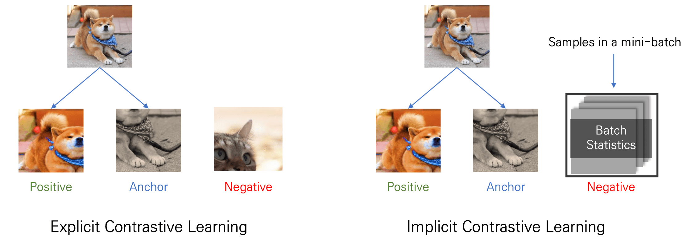
$\mathbf{Fig\ 7.}$ Implicit Contrastive learning by batch statistics
BYOL works even without Batch Statistic
However, Richemond et al. arXiv 2020 experimentally showed that replacing BN with a batch-independent normalization achieves performance comparable to vanilla BYOL, which disproves the hypothesis that the use of batch statistics is a crucial ingredient for BYOL to learn useful representations. They refuted the following hypotheses:
- BN provides an implicit negative term required to avoid collapse
They also observe that removing all BN leads to performance that is no better than random, and consent the hypothesis that BN implicitly introduces a negative contrastive term. However, we observe that BN seems to be mainly useful in the ResNet encoder that standard initializations are known to lead to poor conditioning. Also BYOL might be even more sensitive to improper initialization as it creates its own targets. Based on these observations, they claim that the main contribution of BN is to compensate for improper initialization, rather than implicit negative term.
To mimic the effect of BN on initial scalings and training dynamics, before training, we can compute per-activation BN statistics for each layer by running a single forward pass of the network with BN on a batch of augmented data. Then, remove batch normalization layers, but retain the scale and offset parameters $\gamma$ and $\beta$ trainable, and initialize them as follows: $$ \gamma_{\text {init }}^k=\frac{\gamma_0^k}{\sigma^k} \quad \text { and } \quad \beta_{\text {init }}^k=-\mu^k \cdot \gamma_{\text {init }}^k $$ where $\gamma_{\textrm{init}}^k$ and $\beta_{\textrm{init}}^k$ are the initialization of the additional trainable parameters corresponding to the $k$-th removed BN, and $\mu^k$ and $\sigma^k$ are the batch statistics computed during the first pass for the $k$-th removed BN. Additionally, set $\gamma_0^k = 0$ if the $k$-th removed BN corresponds to the final BN layer in a residual block, and $\gamma_0^k = 1$ otherwise.
The results show that BYOL avoids collapse and achieves good performance without using any normalization during training: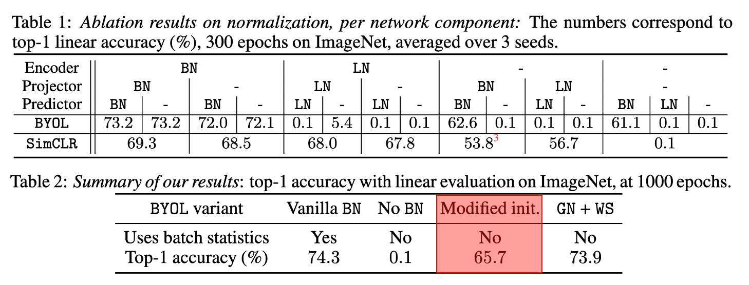
$\mathbf{Fig\ 8.}$ Proper initialization allows working without BN (Richemond et al. 2020)
Consequently, they hypothesize that the principal function of BN is to make the network more robust to cases when the initialization is scaled improperly. Indeed, BYOL encounters challenges from a poor initialization in two ways:- as for any deep network, it makes optimization difficult
- the target network outputs will be ill-conditioned, which initially provides poor targets for the online network.
- BYOL cannot achieve competitive performance without the implicit contrastive effect provided by batch statistics
By using the combination of group normalizing and weight standardization but without batch normalization, they have achieved the performance that rivals those of vanilla BYOL.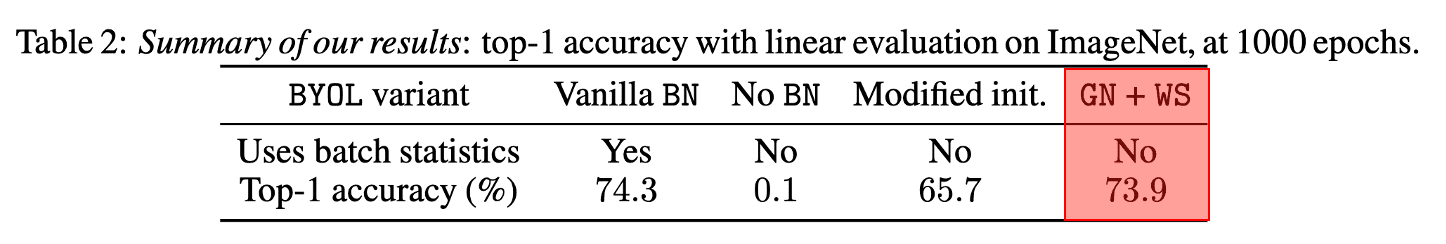
$\mathbf{Fig\ 9.}$ Using GN with WS leads to competitive performance (Richemond et al. 2020)
References
[1] Grill et al. “Bootstrap Your Own Latent A New Approach to Self-Supervised Learning”, NeurIPS 2020
[2] Abe Fetterman, Josh Albrecht, “Understanding self-supervised and contrastive learning with “Bootstrap Your Own Latent” (BYOL)”
[3] Richemond et al., “BYOL works even without batch statistics”, arXiv preprint arXiv:2010.10241.
Leave a comment