[Representation Learning] SimSiam: BYOL without the momentum encoder

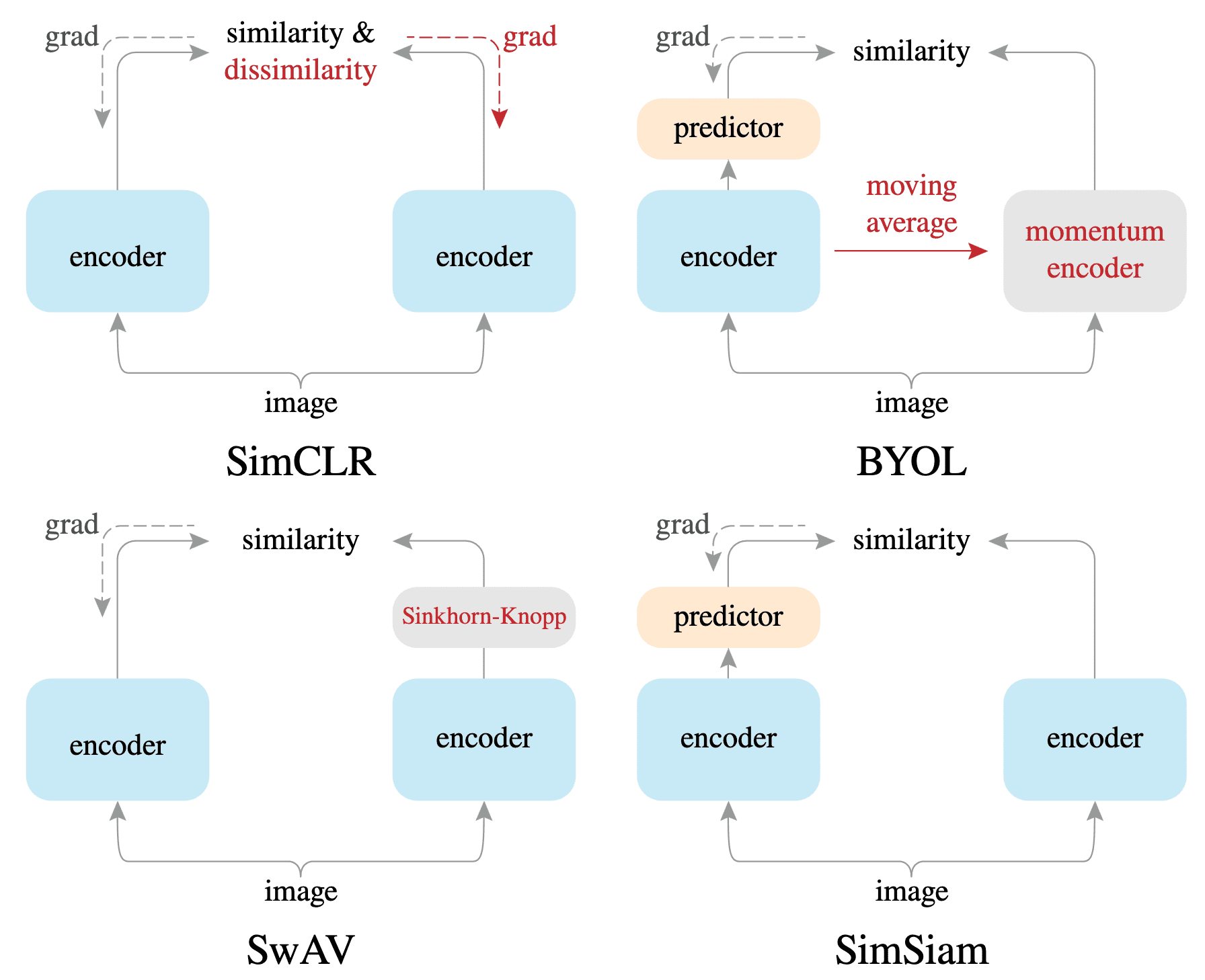
Despite various original motivations, self-supervised learning methods such as SimCLR, BYOL, and SwAV, typcially incorporate certain forms of Siamese networks. Siamese networks, which are weight-sharing neural networks applied to two or more inputs, serve as natural tools for comparing different entities.

However, Siamese networks in representation learning are susceptible to collapsed representation problem, where all encoder outputs collapse to a constant representation for all images. While SimCLR and SwAV avoid the collapse by leveraging negative pairs, BYOL, which operates, without negative pairs, claims to avoid collapse via the use of momentum encoder. SimSiam, introduced by Chen et al. CVPR 2021, claims its collapse avoidance solely through Siamese networks without the need for a momentum encoder.

$\mathbf{Fig\ 1.}$ Comparison on Siamese architectures (Chen et al. 2021)

SimSiam: Simple Siamese Network

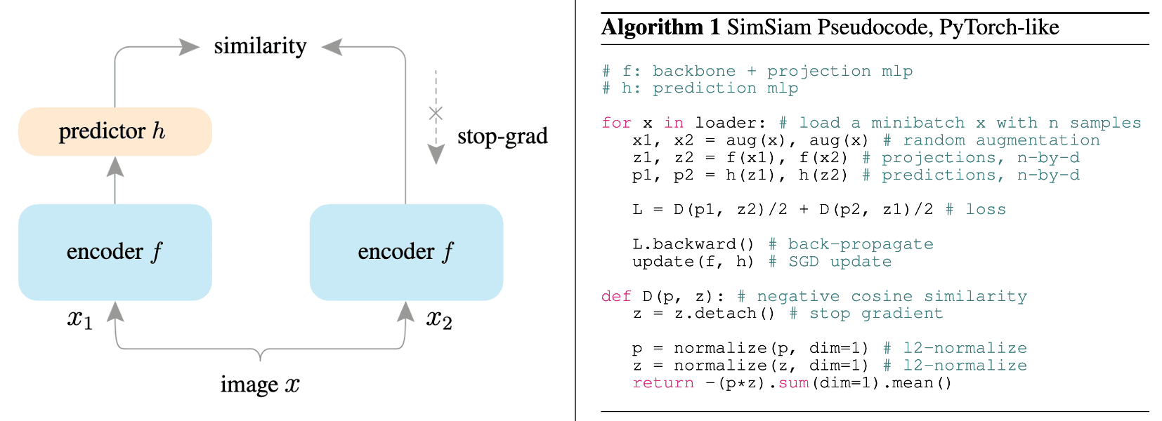
The overall algorithm of SimSiam is explained below:

1. Augmentation
   For given input image $\boldsymbol{x}$, apply two random augmentation and obtain two different views $\boldsymbol{x}_1 = \mathcal{T}_1 (\boldsymbol{x})$ and $\boldsymbol{x}_2 = \mathcal{T}_2 (\boldsymbol{x})$.
2. Predictor & Target networks
   For an encoder network $f$ consisting of a backbone and a projection MLP head, predictor and target network are defined by $h_\phi \circ f_\theta$ where $h_\phi$ is a prediction MLP head and $f_{\theta^\prime}$, respectively. The encoder $f$ of two networks shares weights, i.e., $\theta = \theta^\prime$.
   
   

   

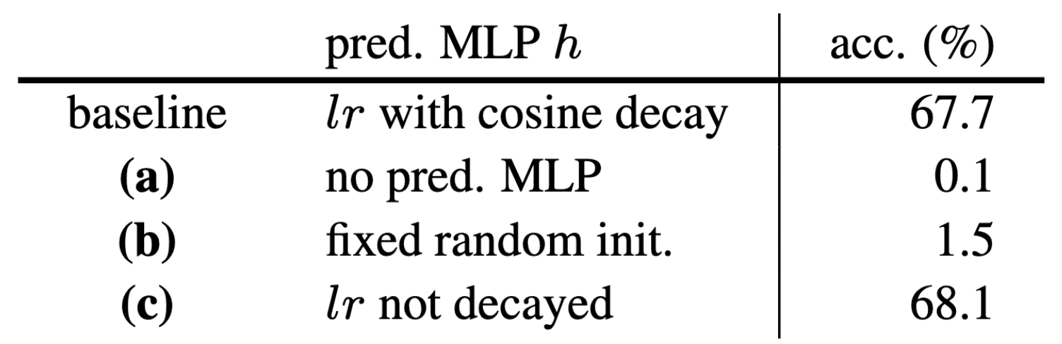
   $\mathbf{Fig\ 3.}$ Effect of prediction MLP $h_\phi$ (Chen et al. 2021)
   
   Then, two views are processed by each two networks: $$ \begin{aligned} \mathbf{p}_1 & = h_\phi (f_\theta (\boldsymbol{x}_1)) \\ \mathbf{p}_2 & = h_\phi (f_\theta (\boldsymbol{x}_2)) \\ \mathbf{z}_1 & = f_{\theta^\prime} (\boldsymbol{x}_2) \\ \mathbf{z}_2 & = f_{\theta^\prime} (\boldsymbol{x}_2) \\ \end{aligned} $$
3. Negative cosine similarity loss
   To avoid finding a degenerated solution (e.g., collapsed representation), the target network is frozen during gradient descent and updated by $\theta^\prime = \theta$ at each iteration.
   
   

   

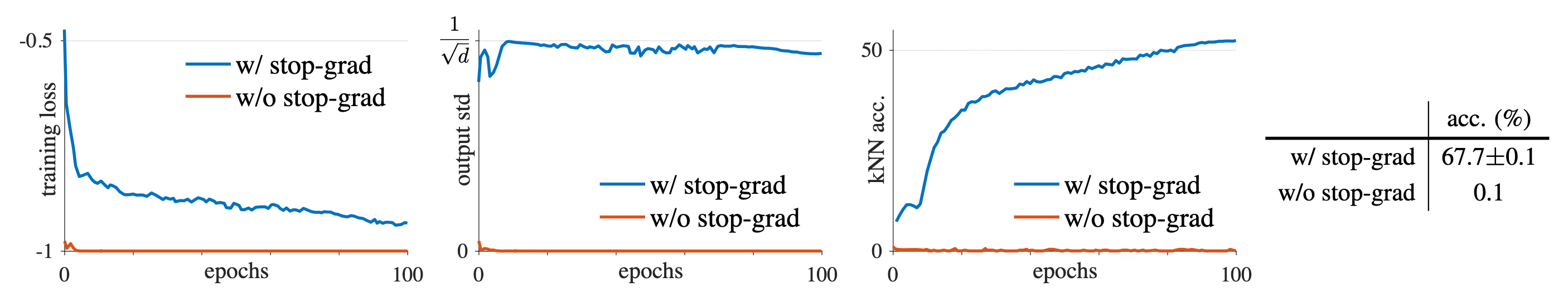
   $\mathbf{Fig\ 3.}$ SimSiam with vs. without stop-gradient (Chen et al. 2021)
   
   And the predictor network $h_\phi \circ f_\theta$ is optimized to minimize the following symmetric loss: $$ \mathcal{L}(\theta) = \frac{1}{2} \mathcal{D} (\mathbf{p}_1, \texttt{stopgrad}(\mathbf{z}_2)) + \frac{1}{2} \mathcal{D} (\texttt{stopgrad}(\mathbf{z}_1), \mathbf{p}_2) $$ where $\mathcal{D}$ is the negative cosine similarity: $$ \mathcal{D} (\mathbf{p}, \mathbf{z}) = - \frac{\mathbf{p}}{\Vert \mathbf{p} \Vert_2} \cdot \frac{\mathbf{z}}{\Vert \mathbf{z} \Vert_2} $$

$\mathbf{Fig\ 4.}$ SimSiam: Simple Siamese Network (Chen et al. 2021)

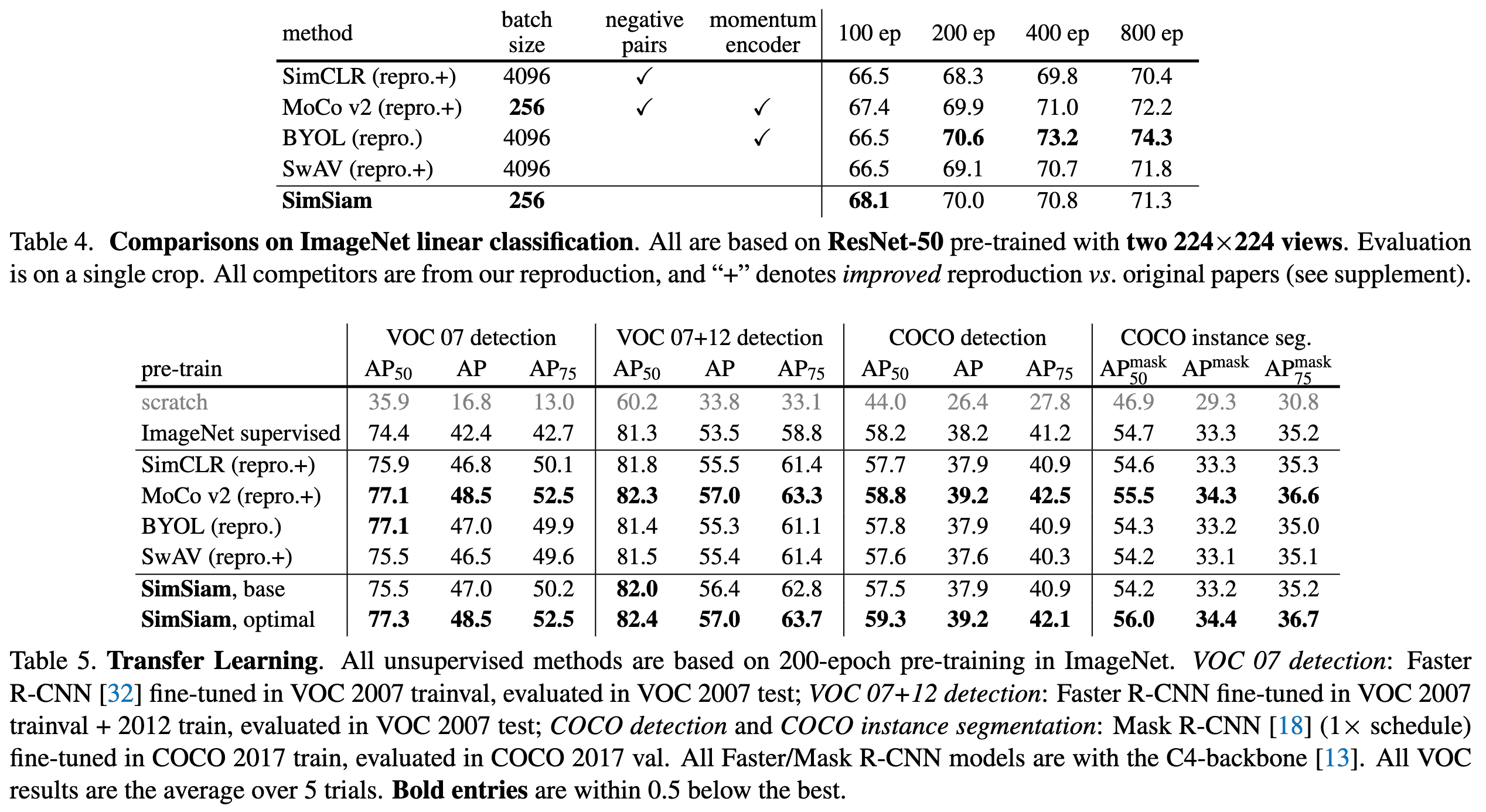
As a result, in ImageNet linear evaluation, SimSiam achieved competitive results with other methods despite its simplicity. Moreover, SimSiam’s representations were highly transferable to other tasks, such as object detection and instance segmentation. This indicates that the Siamese structure is a fundamental factor in the general success of contrastive learning frameworks.

$\mathbf{Fig\ 5.}$ The performance of SimSiam (Chen et al. 2021)

Theoretical Hypothesis

Recall that Expectation-Maximization (EM) algorithm is an iterative algorithm that implicitly involves two sets of variables, and solves the MLE with two underlying sub-problems. The authors hypothesized that SimSiam can be formulated in the form of EM algorithm and verified this through additional experiments.

SimSiam is an Expectation-Maximization (EM) like algorithm

Consider the following loss function:

\[\mathcal{L} (\theta, \mathbf{z}) = \mathbb{E}_{\boldsymbol{x}, \mathcal{T}} [ \Vert \mathcal{F}_\theta (\mathcal{T} (\boldsymbol{x})) - \mathbf{z}_\boldsymbol{x} \Vert_2^2]\]

where

• $\mathcal{F}_\theta$ is a neural network parameterized by $\theta$;
• $\mathcal{T}$ is the augmentation;
• $\mathbf{z}$ is a set of image representation, and $\mathbf{z}_\boldsymbol{x}$ is the representation of an image $\boldsymbol{x}$ accessed using image index;

And consider solving $\underset{\theta, \mathbf{z}}{\min} \; \mathcal{L} (\theta, \mathbf{z})$. Simply, we can solve this optimization problem by an alternating algorithm, fixing one set of variables and solving for the other set. That is, by alternating between solving the following two subproblems:

\[\begin{gathered} \begin{aligned} \theta^t & \leftarrow \underset{\theta}{\arg \min} \; \mathcal{L} (\theta, \mathbf{z}^{t-1}) \\ \mathbf{z}^t & \leftarrow \underset{\mathbf{z}}{\arg \min} \; \mathcal{L} (\theta^t, \mathbf{z}) \\ \end{aligned} \\ \Downarrow \\ \begin{aligned} \theta^t & \leftarrow \theta_t - \alpha \nabla_{\theta} \mathcal{L} (\theta, \mathbf{z}^{t-1}) \\ \mathbf{z}_\boldsymbol{x}^t & \leftarrow \mathbb{E}_\mathcal{T} [ \mathcal{F}_\theta ( \mathcal{T} (\boldsymbol{x} ) )] \end{aligned} \\ \end{gathered}\]

SimSiam can be approximated by one-step alternation of these two update rules. By sampling the augmentation $\mathcal{T}^\prime$ and ignoring $\mathbb{E}_\mathcal{T} [\cdot]$:

\[\begin{aligned} \mathbf{z}_\boldsymbol{x}^t & \leftarrow \mathcal{F}_\theta ( \mathcal{T}^\prime (\boldsymbol{x}) ) = f_{\theta^\prime} (\mathcal{T}^\prime (\boldsymbol{x})) \\ \theta^{t+1} & \leftarrow \underset{\theta}{\arg \min} \; \mathbb{E}_{\boldsymbol{x}, \mathcal{T}} [ \Vert \mathcal{F}_\theta (\mathcal{T} (\boldsymbol{x})) - \mathcal{F}_\theta ( \mathcal{T}^\prime (\boldsymbol{x}) ) \Vert_2^2] \\ & = \underset{\theta}{\arg \min} \; \mathbb{E}_{\boldsymbol{x}, \mathcal{T}} [ \Vert \mathbf{z}_1 - \mathbf{z}_2 \Vert_2^2] \end{aligned}\]

And other components such as prediction MLP head $h_\phi$ and the symmetrization of loss can be involved in this analysis as follows:

• Prediction head $h_\phi$
  The predictor $h_\phi$ is expected to minimize: $$ \mathbb{E}_\mathbf{z} [ \Vert h_\phi (\mathbf{z}_1) - \mathbf{z}_2 \Vert_2^2 ] $$ In other words, the optimal $h$ should satisfy: $$ h(\mathbf{z}_1) = \mathbb{E}_\mathbf{z} [\mathbf{z}_2] = \mathbb{E}_\mathcal{T} [f_{\theta^\prime} ( \mathcal{T} (\boldsymbol{x}))] \; \forall \boldsymbol{x} $$ Hence, the usage of $h$ helps the predictor to approximate $\mathbb{E}_\mathcal{T} [\cdot]$ that we ignored to obtain $\mathbf{z}_\boldsymbol{x}^t$ in the analysis.


• Symmetrization of loss function
  Symmetrization of SimSiam can be regarded as a denser sampling of $\mathcal{T}$. The SGD optimizer computes the empirical expectation $\mathbb{E}_{\boldsymbol{x}, \mathcal{T}} [\cdot]$ by sampling a batch of images with one pair of augmentations $(\mathcal{T}_1, \mathcal{T}_2)$. And here, symmetrization can supply an extra pair $(\mathcal{T}_2, \mathcal{T}_1)$. This explains that symmetrization is not necessary but improves the performance:
  
  

  

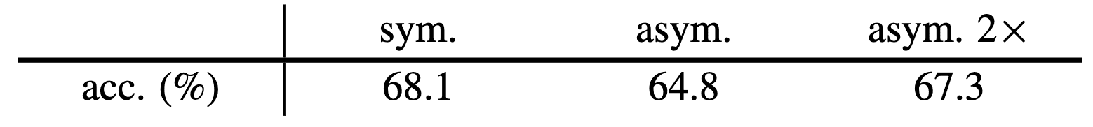
  $\mathbf{Fig\ 6.}$ Performance improvement of Symmetrization (Chen et al. 2021)
  
  

Experimental Proof

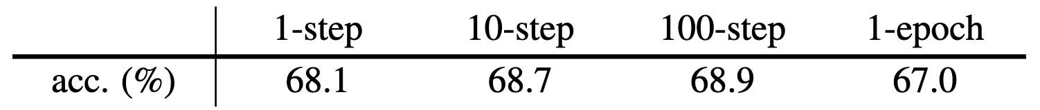
First, to verify the validity of the alternating optimization formulation, the authors experimented the multi-step variants that perform $k$ SGD steps to update $\theta$ and assign $\theta^\prime = \theta$. Notably, $k = 1$ is equivalent to SimSiam. As a result, all multi-step variants performs well and the $k = 10, 100$ variants achieve even better results than SimSiam. This suggests that the alternating optimization is a valid formulation, and SimSiam represents a special case of it.

$\mathbf{Fig\ 7.}$ Performance of multi-step variants (Chen et al. 2021)

The authors hypothesized that the predictor $h_\phi$ is required because the expectation \(\mathbb{E}_\mathcal{T} [\cdot]\) is ignored in the analysis of \(\mathbf{z}_\boldsymbol{x}^t\). To demonstrate this, they attempted to approximate this expectation without the predictor $h_\phi$. Interestingly, they found that momentum encoder for the target network, instead of direct assignment $\theta^\prime = \theta$, can eliminate the need for $h$:

\[\mathbf{z}_\boldsymbol{x}^t \leftarrow \lambda \mathbf{z}_\boldsymbol{x}^{t-1} + (1 - \lambda) \mathcal{F}_{\theta^t} (\mathcal{T}^\prime (\boldsymbol{x}))\]

This variant has $55.0\%$ accuracy without the predictor $h_\phi$, whereas discarding both fails completely. This finding supports that the usage of predictor $h_\phi$ is related to approximating $\mathbb{E}_\mathcal{T} [\cdot]$.

Reference

[1] Chen et al., “Exploring Simple Siamese Representation Learning”, CVPR 2021