[Representation Learning] DINO

DINO: Self-Distillation with NO labels

DINO, self-distillation with no labels introduced by Caron et al. 2021, learns the image representation in the form of knowledge distillation in a self-supervised manner. It employs a non-contrastive loss (i.e., no negative pairs) that relies on the dynamics of learning to avoid collapse.

$\mathbf{Fig\ 1.}$ DINO: Self-distillation with No labels (KamWoh Ng)

The DINO framework consists of 3 major components:

1. Self-distillation
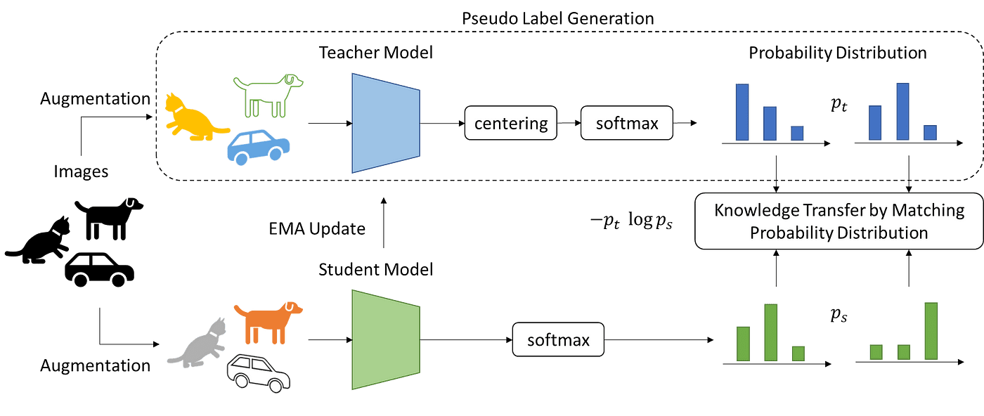
   Knowledge distillation is a learning paradigm where we train a student network $g_{\theta_\texttt{student}}$ to match the output of a given teacher network $g_{\theta_\texttt{teacher}}$, parameterized by $\theta_\texttt{student}$ and $\theta_\texttt{teacher}$ respectively. Both networks consist of a backbone encoder $f$ and a projection head $h$ ($3$-layer MLP), i.e. $g = h \circ f$. Using a cross-entropy loss, DINO distills the teacher, which corresponds to EMA version of a student, knowledge to the student: $$ \begin{gathered} \theta_\texttt{student} \leftarrow \texttt{optimizer}(\theta_\texttt{student} , \nabla_{\theta_\texttt{student}} \mathcal{L}_{\texttt{DINO}}) \\ \theta_\texttt{teacher} \leftarrow \lambda \theta_\texttt{teacher} + (1-\lambda) \theta_\texttt{student} \end{gathered} $$
   Given an input image $\boldsymbol{x}$, the DINO loss is defined as follows: $$ \mathcal{L}_{\texttt{DINO}} = \mathbb{H} (\mathbb{P}_\texttt{teacher} (\boldsymbol{x}), \mathbb{P}_\texttt{student} (\boldsymbol{x})) = - \mathbb{P}_\texttt{teacher} (\boldsymbol{x}) \cdot \log \mathbb{P}_\texttt{student} (\boldsymbol{x}) $$ where both networks output probability distributions using $\texttt{softmax}$: $$ \mathbb{P}_\texttt{student} (\boldsymbol{x})^{(l)} = \texttt{softmax} (g_{\theta_\texttt{student}} (\boldsymbol{x})) = \frac{\exp ( g_{\theta_\texttt{student}} (\boldsymbol{x})^{(l)} / \tau_s )}{ \sum_{k=1}^K \exp ( g_{\theta_\texttt{student}} (\boldsymbol{x})^{(k)} / \tau_s ) } $$ with $\tau_s > 0$ a temperature parameter that controls the sharpness of the output distribution, and a similar formula holds for $\mathbb{P}_\texttt{teacher}$ with temperature $\tau_t$.
   
   
2. Multi-crop
   To generate positive views, DINO constructs a set of views $V$ via multi-crop strategy, which is originally proposed by SwaV paper:
   • (1) global views $\boldsymbol{x}_1^g$, $\boldsymbol{x}_2^g$ (e.g., $> 50\%$ area of the original image)
   • (2) local views with smaller resolution (e.g., $< 50\%$ area of the original image)

   

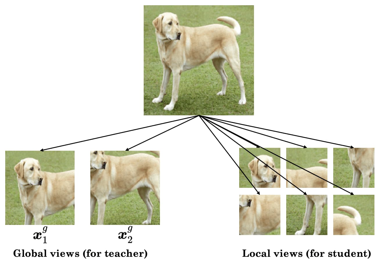
   $\mathbf{Fig\ 2.}$ Multi-crop for DINO
   
   To encourage local-to-global correspondences, all local crops are passed through the student, while only the global views are passed through the teacher. Therefore, $\mathcal{L}_{\texttt{DINO}}$ is finally written as: $$ \mathcal{L}_{\texttt{DINO}} = \sum_{\boldsymbol{x} \in \{ \boldsymbol{x}_1^g, \boldsymbol{x}_2^g \}} \sum_{\begin{gathered} \boldsymbol{x}^\prime \in V \\ \boldsymbol{x}^\prime \neq \boldsymbol{x} \end{gathered}} \mathbb{H} (\mathbb{P}_\texttt{teacher} (\boldsymbol{x}), \mathbb{P}_\texttt{student} (\boldsymbol{x}^\prime)) $$
   
   
3. Centering & Sharpening
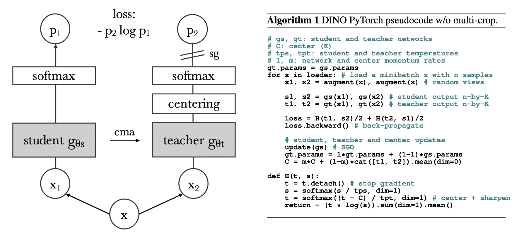
   To avoid collapse, DINO employs centering and sharpening.
   • Centering: adding a bias term $c$ to the teacher output: $$ g_{\theta_\texttt{teacher}} (\boldsymbol{x}) \leftarrow g_{\theta_\texttt{teacher}} (\boldsymbol{x}) + c $$ where the center $c$ is updated with an EMA: $$ c \leftarrow \kappa c + (1 - \kappa) \sum_{i=1}^B g_{\theta_\texttt{teacher}} (\boldsymbol{x}_i) $$ for batch size $B$.
   • Sharpening: using a low value for the temperature $\tau_t$ in the teacher softmax normalization. For example, $\tau_t = 0.04 \to 0.07$ while $\tau_s = 0.1$
   
   Experimentally, centering is essential to prevent collapse to a single dimension, while sharpening is necessary to prevent collapse to a uniform distribution.
   
   

   

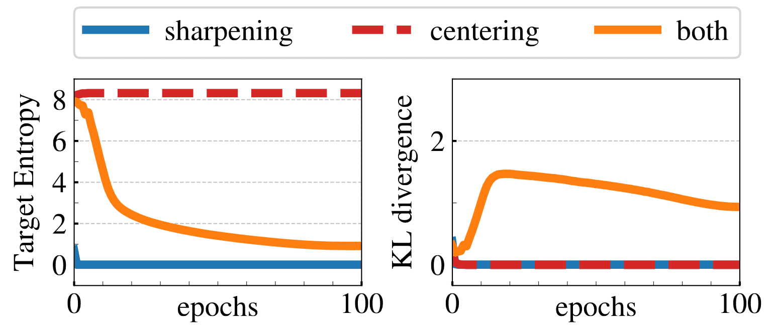
   $\mathbf{Fig\ 3.}$ Collapse study (Caron et al. 2021)
   
   

In summary, the overview of the DINO framework is provided with the pseudocode in the following figure:

$\mathbf{Fig\ 4.}$ DINO overview with pseudocode (Caron et al. 2021)

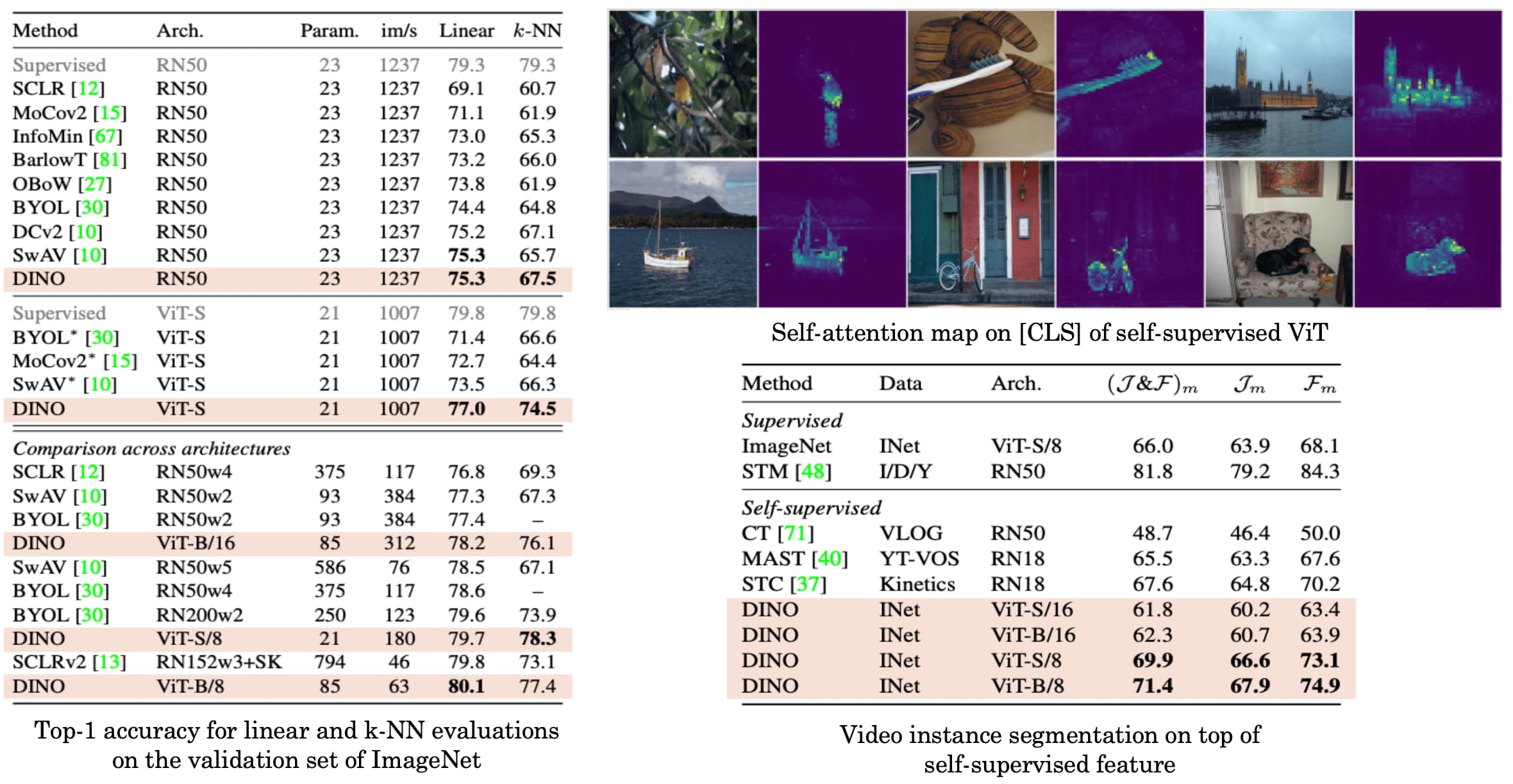
As a result, DINO outperforms previous contrastive methods in classification tasks. Interestingly, self-supervised ViT features contain explicit information about the semantic segmentation of an image, including scene layout and object boundaries. In contrast, supervised ViT does not perform as well in the presence of clutter, both qualitatively and quantitatively.

$\mathbf{Fig\ 5.}$ Experiment Results of DINO (Caron et al. 2021)

DINO v2: Learning Robust Visual Features without Supervision

While recent breakthroughs in self-supervised learning have emerged, CLIP demonstrated better scalability with natural language supervision. DINO v2 aim to scale image-only discriminative self-supervised learning by:

• Scaling data size through curated data;
• Scaling model size with computational efficient engineering techniques;

$\mathbf{Fig\ 6.}$ Linear evaluation on ImageNet-1k of frozen pretrained features (Oquab et al. 2023)

1. Data pre-processing
   The authors curated a dataset termed LVD-142M dataset, which is retrieved from a large pool of uncurated data and images (sourced from crawled web data), that are close to those in several curated datasets (ImageNet and several fine-grained datasets). The data processing pipeline of DINO v2 consists of two key components:
   • Deduplication: To reduce redundancy and increase diversity among images, they removed near-duplicate images;
   • Self-supervised image retrieval: By embedding images with ImageNet-22k pretrained ViT-H/16, they retrieved relevant data from uncurated source that are close to images in the curated sources using $K$-means clustering;
   
   
   

   

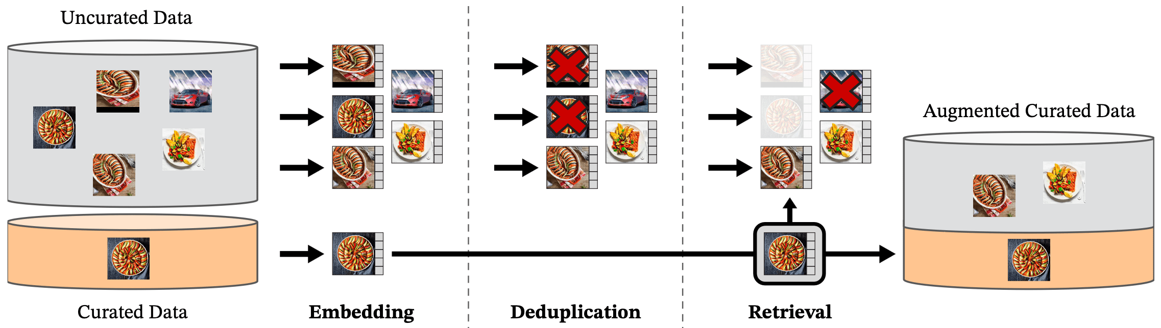
   $\mathbf{Fig\ 7.}$ Overview of DINO v2 data processing pipeline (Oquab et al. 2023)
   
   
2. Discriminative Self-supervised Pre-training
   To leverage longer training with larger batch sizes under large quantity of curated dataset, they designed efficient training methods that learn features at both the image and patch level.
   • Image-level objective: By attaching DINO head on the training encoders, the DINO loss term is computed: $$ \mathcal{L}_{\texttt{DINO}} = - \sum p_\texttt{teacher} \log p_\texttt{student} $$
   • Patch-level objective: By randomly masking some of the input patches given to the student, but not to the teacher, and attaching iBOT head, the iBOT loss term is computed: $$ \mathcal{L}_{\texttt{DINO}} = - \sum_{i \in \mathcal{M}} p_{\texttt{teacher}, i} \log p_{\texttt{student}, i} $$ where $\mathcal{M}$ are patch indices for masked token.
   Note that two different projection heads are separated and do not share parameters. $$ \mathcal{L}_{\texttt{DINOv2}} = \mathcal{L}_{\texttt{DINO}} + \mathcal{L}_{\texttt{iBOT}} + \mathcal{L}_{\texttt{koleo}} $$ To spread features and a short high-resolution training phase, Kozachenko-Leonenk (KoLeo) regularizer is added to the entire loss. It minimizes the differential entropy of features, thereby encouraging features to be uniformly distributed: $$ \mathcal{L}_{\texttt{koleo}} = - \frac{1}{N} \sum_{i=1}^N \log (d_{N, i}) \text{ where } d_{N, i} = \min_{j \neq i} \Vert \boldsymbol{z}_i - \boldsymbol{z}_j \Vert $$
   
   

   

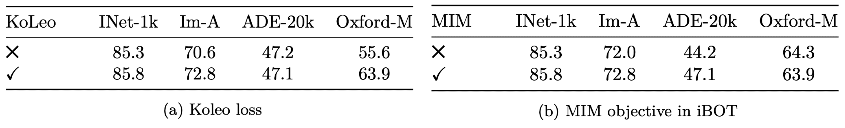
   $\mathbf{Fig\ 8.}$ Effect of KoLeo loss term and MIM from iBOT on Linear Probing (Oquab et al. 2023)
   
   
   
   

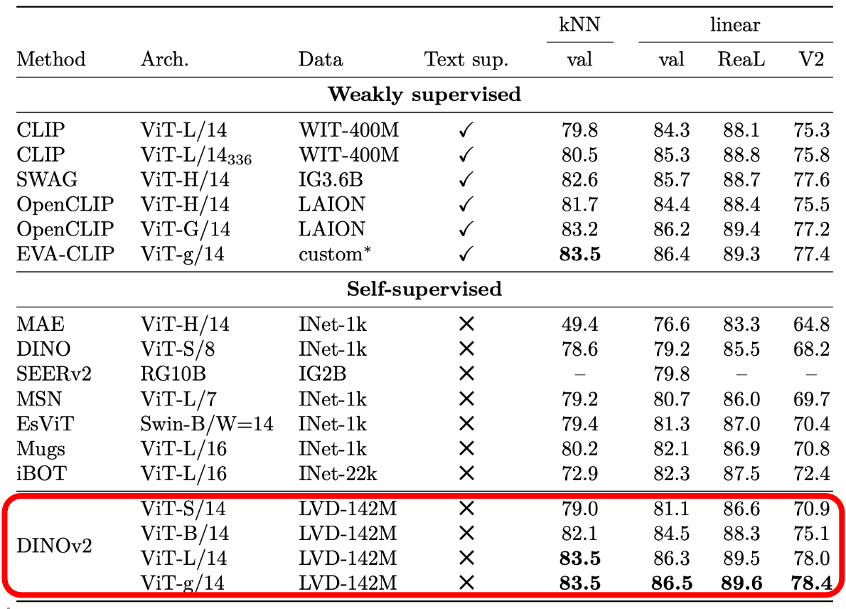
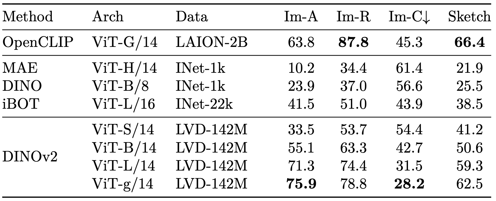
Consequently, DINO v2 matches domain generalization performance of CLIP. When comparing with other state-of-the-art SSL methods on linear probing under ImageNet-A/R/C/Sketch, DINO v2 demonstrates significantly better robustness:

$\mathbf{Fig\ 9.}$ Domain Generalization with a linear probe (Oquab et al. 2023)

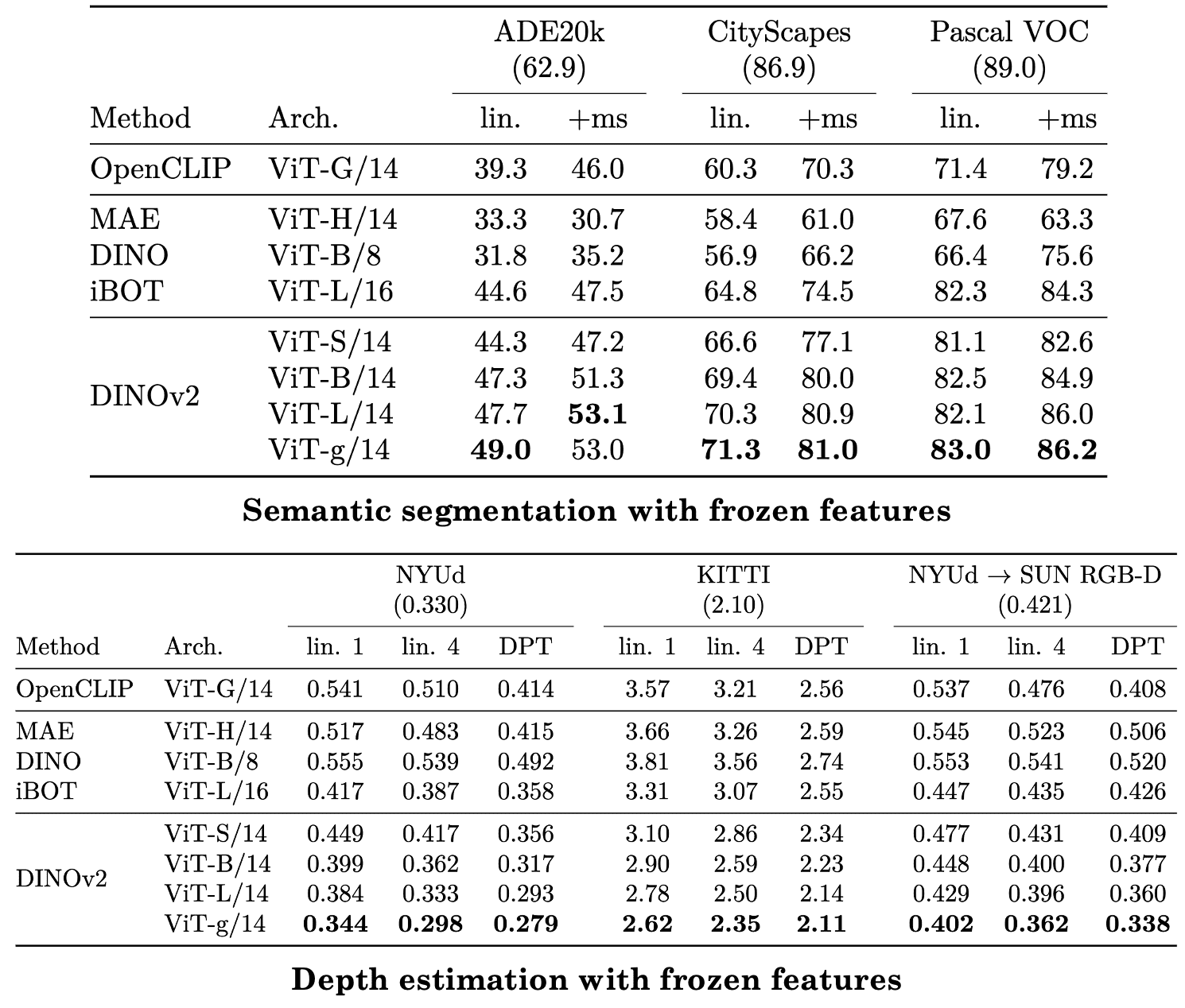
Furthermore, DINO v2 was better at transferring to vision tasks than other methods including CLIP, demonstrating drastically better robustness:

$\mathbf{Fig\ 10.}$ Transfer to vision tasks with frozen features (Oquab et al. 2023)

Reference

[1] Caron et al. “Emerging Properties in Self-Supervised Vision Transformers”, ICCV 2021
[2] Oquab et al. “DINOv2: Learning Robust Visual Features without Supervision”, arXiv 2023