
[Representation Learning] Clustering Visual Features
Introduction
The general contrastive learning methods necessitate numerous explicit pairwise comparisons with negative pairs, rendering them computationally daunting. Consequently, it demands the careful treatement to retrieve a large volume of negative pairs, exemplified by memory banks in MoCo, batch size in SimCLR. And since computing all the pairwise comparisons on a large dataset is not practical, this is one of the motivations behind BYOL that obviates the necessity of negative pairs in learning visual features, as we saw in the previous post.
In contrast, clustering-based representation learning offers an alternative approach to relax the instance discrimination problem. The objective of clustering-based methods is to gather images with similar representations into clusters, enabling discrimination between cluster assignments rather than individual images or representations, thereby notably enhancing efficiency. (It is also possible to create the labels in an unsupervised fashion.) Over the time, numerous clustering-based methods have been developed, each possessing its own strengths and weaknesses. And we’ll discuss the most significant approaches in this post.
DeepCluster
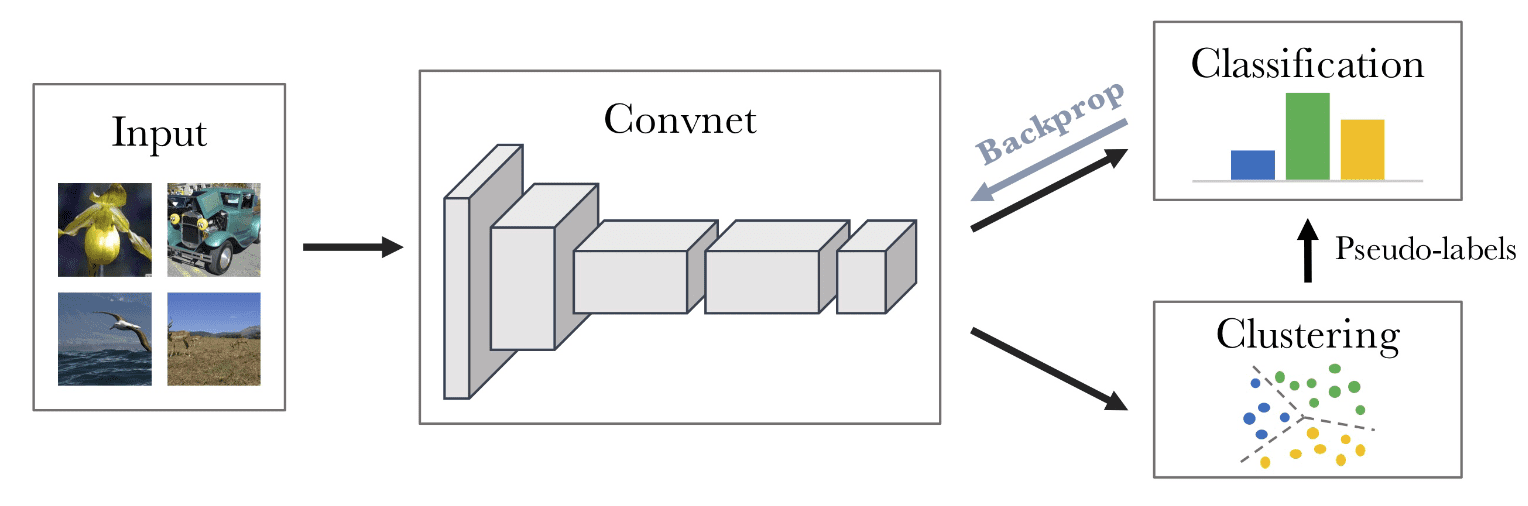
DeepCluster (Caron et al. ECCV 2018) iteratively learns the features and clusters them: alternates between clustering of the visual features and updating the weights of the convnet by predicting the cluster assignment as pseudo-label.
Given the encoder $f_\theta: \mathcal{I} \to \mathbb{R}^{d}$, it jointly learns a centroid matrix $\mathbf{M} \in \mathbb{R}^{d \times k}$ and the cluster assignments $\boldsymbol{y}_n \in \mathbb{R}^k$ of each image $\boldsymbol{x}_n$ by solving the optimization problem:
\[\min_{\mathbf{M} \in \mathbb R^{d\times k}}\frac {1}{N}\sum^N_{n=1}\min_{\boldsymbol{y}_n\in\{0,1\}^k} \lVert f_\theta(\boldsymbol{x}_n)- \mathbf{M} \boldsymbol{y}_n \rVert^2_2 \qquad \text{such that} \qquad \boldsymbol{y}_n^\top \mathbf{1}_k=1 \tag 1\]Solving this problem provides a set of optimal assignments \(\{\boldsymbol{y}_n^*\}_{n \leq N}\) and a centroid matrix $C^*$. Let $g_\phi: \mathbb{R}^d \to \mathbb{R}^k$ be a parametrized classifier that predicts the correct labels on top of the features $f_\theta (\boldsymbol{x}_n)$. Then, with the cluster assignments obtained from the previous optimization problem, the classifier and the encoder are jointly learned by solving the following problem:
\[\min_{\theta, \phi} \frac {1}{N}\sum^N_{n=1}\mathcal{L}(g_\phi \circ f_\theta(\boldsymbol{x}_n),\boldsymbol{y}_n) \tag 2\]In their experiments, the authors utilize a standard AlexNet with k-means for clustering and claim that the choice of the clustering algorithm is not crucial. However, this iterative procedure is prone to trivial solutions; DeepCluster requires extra techniques to avoid such degenerate solutions:
- Empty clusters: The algorithm can assign all of the inputs to a single cluster. To overcome this issue, we can randomly select a non-empty cluster, perturbs its centroid with a small random noise as the new centroid, and then reassign the points belonging to the non-empty cluster to the two resulting clusters.
- Trivial parametrization: Highly unbalanced class distribution might lead to a trivial parametrization where the convnet will predict the same output regardless of the input. To overcome this issue, sample images based on a uniform distribution over the classes, or pseudo-labels. Equivalently, weight the contribution of an input to the loss function by the inverse of the size of its assigned cluster.
DeeperCluster
Motivation
The widely used datasets such as ImageNet are made of carefully selected images by human, therby being well-balanced and diversified. Hence, it leads to a significant degradation of the quality of features in unsupervised situations as large-scale non-curated data requires model complexity to increase with dataset size and stability to data distribution changes.
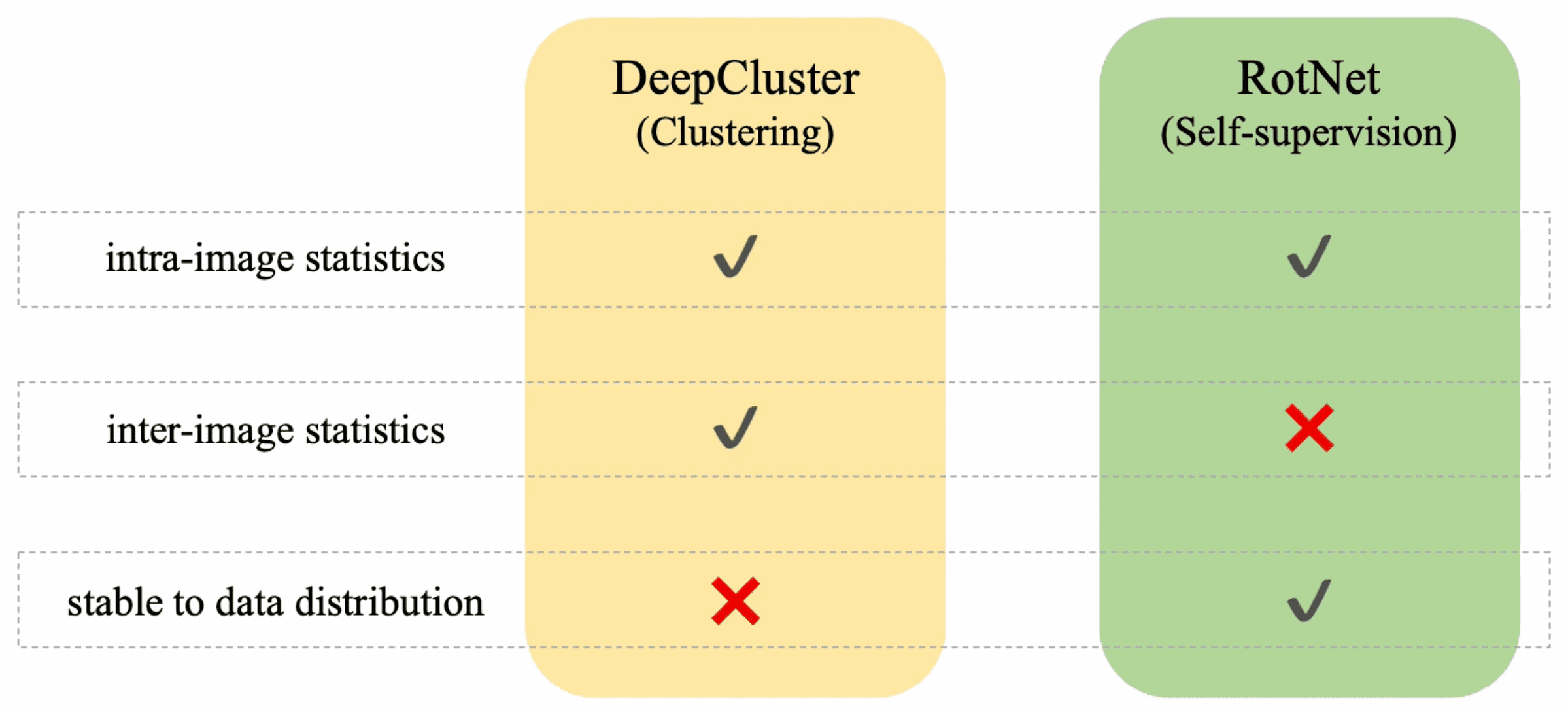
Although clustering-based methods are scalable; can capture much finer relations between images when the number of clusters scales with the dataset, DeepCluster is highly unstable as it simultaneously infers target labels and learns visual features. Moreover, these methods are sensitive to data distribution as they rely directly on cluster structure constructed upon the input dataset.
In contrast, a self-supervised learning approach such as RotNet that formulates the multi-class prediction problem to predict degree of rotation applied to the input image leverages intra-image statistics to build supervision without class information. Hence, RotNet is often independent of the data distribution and thus it is stable to distribution change.
Algorithm
Inspired by these works, Caron et al. 2019 combines two approaches and designs a new self-supervised approach to leverage large amount of raw data, termed DeeperCluster. It alternates between a hierachical clustering of the features and learning the encoder by predicting both the rotation angle and the cluster assignments in a single hierachical loss.
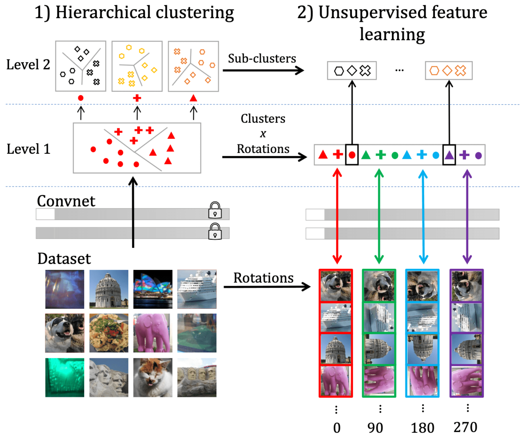
Combining two approaches by summing two losses implicitly assumes that classifying rotations and cluster memberships are two independent tasks, which may limit the signal that can be captured. Instead, DeeperCluster predicts the Cartesian product space of rotation angle and the cluster assignments $\mathcal{Y} \times \mathcal{Z}$ to capture richer interactions between the two tasks.
Assume that the inputs \(\boldsymbol{x}_1, \cdots, \boldsymbol{x}_N\) are rotated images, each associated with a target label $y_n \in \mathcal{Y}$ (e.g. \(\mathcal{Y} = \{0^\circ, 90^\circ, 180^\circ, 270^\circ\}\)) that indicates its rotation angle and a cluster assignment \(\boldsymbol{z}_n \in \mathcal{Z}\) (e.g. \(\mathcal{Z} = \{0, 1\}^k\)). For the encoder $f_\theta$ and the classifier head $g_\phi$, DeeperCluster aims to solve the following optimization:
\[\min_{\theta, \phi} \frac {1}{N}\sum^N_{n=1}\mathcal{L}(g_\phi \circ f_\theta(\boldsymbol{x}_n), y_n \otimes \boldsymbol{z}_n) \tag 3\]However, this formulation does not scale in the number of combined targets as its complexity is $O(\vert \mathcal{Y} \vert \vert \mathcal{Z} \vert)$. Instead, DeeperCluster provides an approximation of this formulation based on a scalable hierarchical loss, with 2-level hierarchy of the target labels. It does so by alternating the following two steps:
- Hierarchical clustering
Given a rotated image $\boldsymbol{x}_n$, it first predicts super-class $\boldsymbol{y}_n \in \{0, 1\}^{S = 4m}$ among Cartesian product between the assignment to these $m$ clusters and 4 angle rotation classes. This is predicted by linear classifier head $h_{\phi}$ on top of the encoder $f_\theta$.
The second-level of the hierarchy is obtained by partitioning within each super-class. Note that there are $S=4m$ super-classes, each associated with the subset of data belonging to the corresponding cluster. These subsets are then further split with $k$-means into $k$ sub-classes. Denote by $\boldsymbol{z}_n^s \in \{0, 1\}^{k}$ the assignment vector into $k$ sub-classes for a rotated image $\boldsymbol{x}_n$ belonging to super-class $s$. For each super-class, $\boldsymbol{z}_n^s$ is predicted by linear classifier head $g_{w_s}$ on top of the encoder $f_\theta$. - Unsupervised feature learning
All parameters for classifiers and encoder are jointly learned by minimizing the following loss: $$ \mathcal{L} = \frac{1}{N} \sum_{n=1}^N\left[\ell\left(g_\phi \circ f_\theta\left(\boldsymbol{x}_n \right), \boldsymbol{y}_n \right)+\sum_{s=1}^S \boldsymbol{y}_{ns} \ell\left(g_{w_s} \circ f_\theta\left(\boldsymbol{x}_n\right), \boldsymbol{z}_n^s\right)\right] \tag 4 $$ where $\ell$ is the negative log-softmax function.
Self-Labelling (SeLa)
Motivation
Combining representation learning, which is a discriminative task, with clustering presents challenges. Typically, in particular DeepCluster that blends the cross-entropy minimization and K-means, lack a singular, well-defined objective to optimize, complicating the characterization of their convergence properties. Besides, DeepCluster is prone to degenerate solutions, wherein all data points are assigned to the same cluster or where a constant representation is learned. Achieving a simultaneous minimization of the cross-entropy loss and the K-means loss necessitates cumbersome heuristics, such as inverse sampling of training data based on their associated cluster sizes.
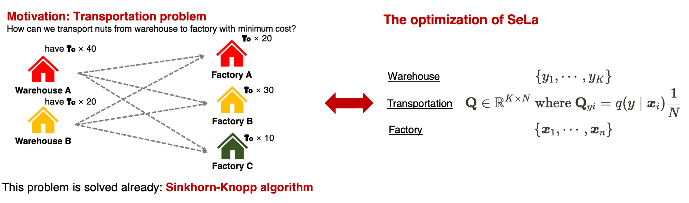
SeLa, introduced by Asano et al. ICLR 2020, offers a principled formulation for simultaneous clustering and representation learning that minimizes the single cross-entropy loss, treating the label assignment problem as optimal transport. Furthermore, SeLa explicitly circumvents degenerate solutions by imposing a straightforward constraint of equipartition, wherein the labels must induce an equal partitioning of the data. This constraint can be seamlessly integrated into the label assignment problem while maintaining the cross-entropy as objective, using a single scalable iterative algorithm called Sinkhorn-Knopp algorithm (Cuturi et al., NIPS 2013).
Formulation
For given $N$ datapoints \(\{I_1, \cdots, I_N\}\) denote $\Phi: \mathbb{R}^{H \times W} \to \mathbb{R}^D$ by feature extractor that yields feature vector $\boldsymbol{x} = \Phi(I)$ from image $I$ and $h: \mathbb{R}^D \to \mathbb{R}^K$ by its classification head, where $K$ is the number of possible labels. SeLa is achieved by jointly optimizing the following objective
\[E(p, q) = - \frac{1}{N} \sum_{i=1}^N \sum_{y=1}^K q(y \mid \boldsymbol{x}_i) p(y \mid \boldsymbol{x}_i) \tag 5\]with respect to the model $h \circ \Phi$ and the labels $y_1, \cdots, y_N$:
\[\min _{p, q} E(p, q) \quad \text { subject to } \quad \forall y: q\left(y \mid \boldsymbol{x}_i\right) \in\{0,1\} \text { and } \sum_{i=1}^N q\left(y \mid \boldsymbol{x}_i\right)=\frac{N}{K} \tag 6\]where \(p(y \mid \boldsymbol{x}_i) = \textrm{softmax}(h \circ \Phi(\boldsymbol{x}_i)) \in \mathbb{R}^K\). Note that the posterior $q(y\vert\boldsymbol{x}_i)$ is encoding of the labels and introduced to avoid the degeneracy that assigning all data points to a single arbitrary label in the fully unsupervised setting, e.g. the optimal setting of $q$ is $q(y\vert \boldsymbol{x}_i) = \delta(y−y_i)$ where $\delta$ denotes Kronecker delta and $y_i$ is true (but might be unknown) label. And to avoid another degeneracy occurs from the optimization of $q$ that is equivalent to reassigning the labels, we add the constraint to $q$. The constraints mean that each data point $\boldsymbol{x}_i$ is assigned to exactly one label and that, overall, the $N$ data points are split uniformly among the $K$ classes. Moreover, the deterministic setting of $q(y\vert\boldsymbol{x}_i)$ leads to the equivalence of objective to the average cross-entropy loss in semi-supervised learning in the sense that:
\[E(p, q) \equiv \mathcal{L}_{\textrm{CE}} = - \frac{1}{N} \sum_{i=1}^N p(y_i \mid \boldsymbol{x}_i) \quad \text{ when } \quad q (y \mid \boldsymbol{x}_i) = \delta(y − y_i) \tag 7\]Algorithm
Then how can we solve the constrained optimization problem that typical backpropagation is inavailable? SeLa designed it as optimal transport problem by considering the cluster labels as supply points, predicted probability $p$ as transportation costs, and the features as demand points; see appendix for the introduction of transport problem. We define matrices \(\mathbf{P}, \mathbf{Q} \in \mathbb{R}_+^{K \times N}\) where \(\mathbf{P}_{yi} = p(y\vert\boldsymbol{x}_i)\) and \(\mathbf{Q}_{yi} = q(y\vert\boldsymbol{x}_i)\). Then, $\mathbf{Q}$ corresponds to the transportation plan, i.e. an element of the transportation polytope
\[U(r, c) := \{ \mathbf{Q} \in \mathbb{R}_+^{K \times N} \mid \mathbf{Q} \mathbf{1} = r, \mathbf{Q}^\top \mathbf{1} = c \} \textrm{ where } r = \frac{N}{K} \cdot \mathbf{1}, c = \mathbf{1} \tag 8\]Or, equivalently, we can also consider the normalized version of the problem with \(\mathbf{P}_{yi} = p(y\vert\boldsymbol{x}_i) \frac{1}{N}\), \(\mathbf{Q}_{yi} = q(y\vert\boldsymbol{x}_i) \frac{1}{N}\) and
\[U(r, c) := \{ \mathbf{Q} \in \mathbb{R}_+^{K \times N} \mid \mathbf{Q} \mathbf{1} = r, \mathbf{Q}^\top \mathbf{1} = c \} \textrm{ where } r = \frac{1}{K} \cdot \mathbf{1}, c = \frac{1}{N} \cdot \mathbf{1} \tag 8\]
Note that the available quantities $r$ and required quantities $c$ are set based on our constraint. Therefore, now it suffices to solve the linear problem
\[\min _{\mathbf{Q} \in U(r, c)}\langle \mathbf{Q},-\log \mathbf{P}\rangle \tag 9\]since $E(p, q) + \log N = \langle \mathbf{Q},-\log \mathbf{P}\rangle$ where $\langle \cdot \rangle$ is the Frobenius inner product between two matrices. Hence it is solvable in polynomial time with linear programming. For scalability with data points and classes, instead SeLa adopts Sinkhorn-Knopp algorithm proposed in Cuturi et al. 2013 see appendix for the brief introduction of transport problem. This algorithm is possible to iteratively solve the equivalent objective that regularization term is introduced
\[\min _{\mathbf{Q} \in U(r, c)}\langle \mathbf{Q},-\log \mathbf{P}\rangle + \frac{1}{\lambda} \textrm{KL}(\mathbf{Q} \| rc^\top) \tag{10}\]and the minimizer amounts to
\[\mathbf{Q} = \textrm{diag}(\alpha) \mathbf{P}^\lambda \textrm{diag}(\beta) \tag{11}\]where $\lambda$ is regularization constant, and $\alpha \in \mathbb{R}^{K}$ and $\beta \in \mathbb{R}^{N}$ are two scaling vectors that normalize the resulting matrix $\mathbf{Q}$ to be probability matrix. All of these factors are found by iterating the updates $\alpha_y \leftarrow [P^\lambda \beta]_y^{-1}$ and $\beta_i \leftarrow [\alpha^\top P^\lambda]_i^{-1}$ that involves a single matrix-vector multiplication with complexity $\mathcal{O}(NK)$, i.e. scales linearly and short convergence time in practice. Finally, note that for very large $\lambda$, optimizing eq. $(10)$ is of course equivalent to optimizing eq. $(9)$. But Cuturi et al. 2013 demonstrates that even for moderate values of $\lambda$ the two objectives tend to have approximately the same optimizer. This is because of trades-off in $\lambda$ between convergence speed and closeness to the original transport problem.
In summary, SeLa is trained by alternating the following two steps:
- Representation Learning
Given the current (fixed) label assignments $Q$, update the parameters $\boldsymbol{\theta}$ of model $h \circ \Phi$ by minimizing the cross-entropy: $$ \tilde{\boldsymbol{\theta}}^* = \underset{\boldsymbol{\theta}}{\textrm{arg min}} -\frac{1}{N} \sum_{y=1}^K \sum_{i=1}^N q (y \vert \boldsymbol{x}_i) p (y \vert \boldsymbol{x}_i) \tag{12} $$ - Self-Labelling.
Given the current model $h \circ \Phi$, we compute the log probabilities $\mathbf{P}$. Then, we find $\mathbf{Q}$ by iterating the updates $$ \begin{aligned} \forall y: & \quad \alpha_y \leftarrow [P^\lambda \beta]_y^{-1} \\ \forall i: & \quad \beta_i \leftarrow [\alpha^\top P^\lambda]_i^{-1} \end{aligned} \tag{13} $$
Of course, SeLa can be further extended to multi-label setting using multiple heads $h_1, \cdots, h_T$ for each of $T$ clustering tasks and optimize a sum of objective functions.
Theoretical Interpretation
This section elucidates that the formulation of SeLa can be construed as the maximization of mutual information between data indices and labels, while concurrently enforcing the equipartition condition—an aspect implicitly implied by maximizing information in any scenario. Contrastingly, minimizing entropy alone may lead to degenerate solutions, as such solutions lack mutual information between labels $y$ and indices $i$. By maximizing information, SeLa effectively mitigates this issue.
Interpret the data index $i$ as a random variable with uniform distribution $p(i) = q(i) = 1/N$ and rewrite $p(y \vert \boldsymbol{x}_i) = p(y \vert i)$ and $q(y \vert \boldsymbol{x}_i) = q(y \vert i)$. Then our objective is turned out to be the cross-entropy between the joint label-index distributions $q(y, i)$ and $p(y, i)$:
\[E(p, q) + \log N = - \sum_{i=1}^N \sum_{y=1}^K q(y, i) \log p (y, i) = H (q, p) = \textrm{KL} (q \vert p) + H (q) \tag{14}\]Hence the minimum of this quantity w.r.t. $q$ is entropy $H_{q} (y, i)$ of the random variables $y$ and $i$ achieved when $p = q$. And the marginal entropy $H_q (i) = \log N$ is constant and, due to the equipartition condition $q(y) = 1/K$, $H_q (y) = \log K$ is also constant. Subtracting these two constants yields:
\[\begin{aligned} \min _p E(p, q)+\log N & = E(q, q)+\log N \\ & = H_q(y, i) = H_q(y)+H_q(i)-I_q(y, i) \\ & = C -I_q(y, i) \propto = -I_q(y, i) \end{aligned} \tag{15}\]Thus we proved that minimizing $E(p, q)$ is equivalent to maximizing the mutual information between the label $y$ and the data index $i$, i.e. maximizing the reduction of the uncertainty of data index $i$ obtained by telling the cluster label $y$.
SwAV
Motivation
The objective in clustering is tractable, but it is not scalable with respect to the dataset. Because they are offline in the sense that they alternate between a cluster assignment, which requires a pass over the entire dataset to form image codes (i.e., cluster assignments), and a training step that codes are used as targets during training.
SwAV (Swapping Assignments between multiple Views of the same image, Caron et al. NeurIPS 2020) use a different paradigm that computes the codes online while enforcing consistency between codes obtained from views of the same image. It scales to potentially unlimited amounts of data, and also works with small and large batch sizes, not necessitating large memory bank or momentum encoder.
Formulation
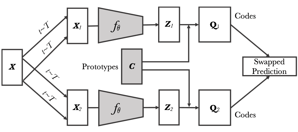
SwAV computes a code from an augmented version of the image and predict this code from other augmented versions of the same image. Given two image features \(\mathbf{z}_t\) and \(\mathbf{z}_s\) from two different augmentations of the same image $\mathbf{x}$, we compute their codes \(\mathbf{q}_t\) and \(\mathbf{q}_s\) by matching these features to a set of prototypes \(\{\mathbf{c}_1, \cdots , \mathbf{c}_K \}\). Then it setups a swapped prediction problem with the following loss function:
\[\mathcal{L} (\mathbf{z}_t, \mathbf{z}_s) = \ell (\mathbf{z}_t, \mathbf{q}_s) + \ell(\mathbf{z}_s, \mathbf{q}_t) \tag{16}\]where $\ell(\mathbf{z}, \mathbf{q})$ measures the fit between features $\mathbf{z}$ and a code $\mathbf{q}$. This problem enforces consistency between codes from different augmentations of the same image.
Algorithm
- Typical feature projection
Each image $\mathbf{x}_n$ is transformed into an augmented view $\mathbf{x}_{nt}$ by applying a transformation $t \sim \mathcal{T}$. The augmented view is mapped to a vector representation by applying a non-linear mapping $f_\theta$ to $\mathbf{x}_{nt}$. Then it is projected to the unit sphere: $$ \mathbf{z}_{nt} = \frac{f_{\theta} (\mathbf{x}_{nt})}{\lVert f_{\theta} (\mathbf{x}_{nt}) \rVert_2} \tag{17} $$ - Online Clustering
Given $B$ feature vectors $\mathbf{Z} = [\mathbf{z}_1, \cdots, \mathbf{z}_B]$ and $K$ trainable prototypes $\mathbf{C} = [\mathbf{c}_1, \cdots, \mathbf{c}_K]$ shared across batch, it generates $B$ codes $\mathbf{Q} = [\mathbf{q}_1, \cdots, \mathbf{q}_B]$ that maps each features to one prototypes by maximizing the similarity between the features and the prototypes. To avoid trivial solution where every image has the same code, SwAV also constraints the codes such that all the examples in a batch are equally partitioned by the prototypes.
Identical to SeLa SwAV models the clustering problem as the transportation problem, finding the optimal $\mathbf{Q}$ from the following optimization problem $$ \begin{aligned} & \underset{\mathbf{Q} \in \mathcal{Q}}{\max} \left[ \langle \mathbf{Q}, \mathbf{C}^\top \mathbf{Z} \rangle + \varepsilon \mathbb{H} (\mathbf{Q}) \right] \\ = & \underset{\mathbf{Q} \in \mathcal{Q}}{\max} \left[ \textrm{Tr} \left(\mathbf{Q}^\top \mathbf{C}^\top \mathbf{Z} \right) + \varepsilon \mathbb{H} (\mathbf{Q}) \right] \end{aligned} \tag{18} $$ with transportation polytopes $$ \mathcal{Q} = \left\{ \mathbf{Q} \in \mathbb{R}_+^{K \times B} \; \middle| \; \mathbf{Q} \mathbf{1} = \frac{1}{K} \mathbf{1}, \mathbf{Q}^\top \mathbf{1} = \frac{1}{B} \mathbf{1} \right\} \tag{19} $$ Note that our cluster assignments (codes) aim to maximize the similar between the similarity $\mathbf{C}^\top \mathbf{Z}$, $\mathbf{C}^\top \mathbf{Z}$ is designed as the negative cost in the corresponding transportation scenario.
Then, from the Sinkhorn distance, the optimal continuous codes $\mathbf{Q}^*$ takes the form of $$ \mathbf{Q}^* = \textrm{diag}(\mathbf{u}) \exp \left( \frac{\mathbf{C}^\top \mathbf{Z}}{\varepsilon} \right) \textrm{diag}(\mathbf{v}) \tag{20} $$ which can be computed iteratively through scalable Sinkhorn-Knopp algorithm: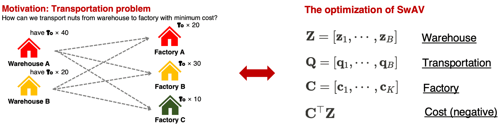
$\mathbf{Fig\ 8.}$ Transportation analogy of SwAV (source: current author)
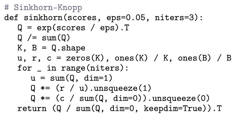
$\mathbf{Fig\ 9.}$ Pseudo-code of Sinkhorn-Knopp for SwAV (Caron et al. 2020) - Swapped prediction
The parameter of model $\theta$ and prototypes $\mathbf{C}$ are optimized by solving the swapped prediction problem of predicting the code $\mathbf{q}_t$ from the feature $\mathbf{z}_s$ and $\mathbf{q}_s$ from $\mathbf{z}_t$: $$ \underset{\theta, \mathbf{C}}{\min} \mathcal{L} (\mathbf{z}_t, \mathbf{z}_s) = \underset{\theta, \mathbf{C}}{\min} \left[ \ell (\mathbf{z}_t, \mathbf{q}_s) + \ell(\mathbf{z}_s, \mathbf{q}_t) \right] \tag{21} $$ where $$ \ell (\mathbf{z}_{t} \mathbf{q}_s) = - \sum_{k=1}^K \mathbf{q}_s^{(k)} \log \mathbf{p}_t^{(k)} \quad \textrm{ where } \quad \mathbf{p}_t^{(k)} = \frac{\exp (\mathbf{z}_t^\top \mathbf{c}_k / \tau)}{\sum_{k^\prime = 1}^K \exp (\mathbf{z}_t^\top \mathbf{c}_{k^\prime} / \tau)} \tag{22} $$
Result
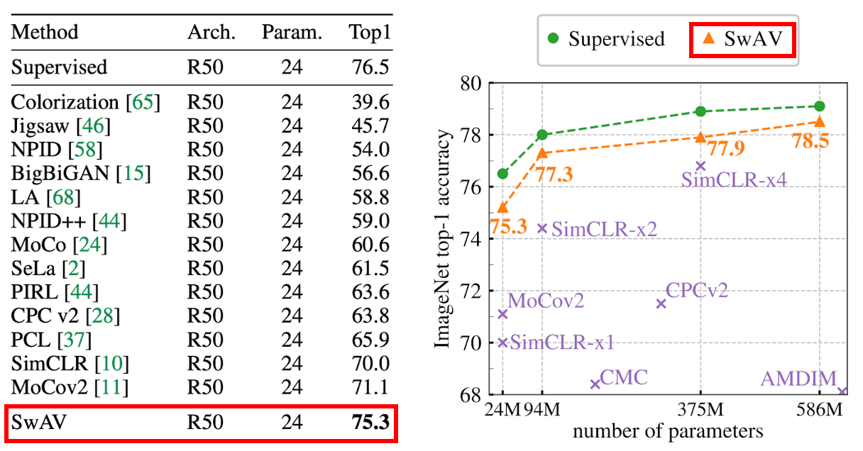
The authors evaluate the features of a ResNet-50 trained with SwAV on linear classification task on frozen features. SwAV outperforms the previous state-of-the-art by +4.2% top-1 accuracy and is only 1.2% below the performance of a fully supervised model.
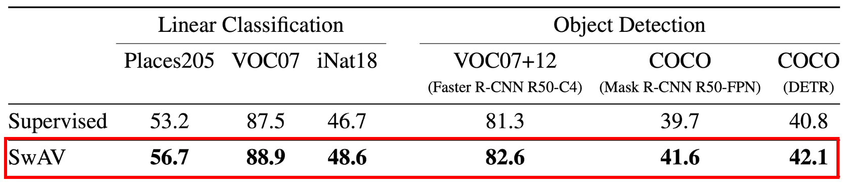
Moreover, to test the generalization of ResNet-50 features trained with SwAV on ImageNet (without labels), the authors transfer these unsupervised features to several downstream vision tasks. They demonstrate that SwAV outperforms the supervised pretrained model on all datasets considered in the experiments, including object detection task.
For more details about SwAV, please refer to the original paper!
Reference
[1] Caron et al., “DeepCluster: Deep Clustering for Unsupervised Learning of Visual Features”, ECCV 2018
[2] Caron et al., “DeeperCluster: Unsupervised Pre-Training of Image Features on Non-Curated Data”, ICCV 2019
[3] Asano et al., “Self-labelling via simultaneous clustering and representation learning”, ICLR 2020
[4] Cuturi et al., “Sinkhorn Distances: Lightspeed Computation of Optimal Transportation Distances”, NIPS 2013
[5] Villani, C. (2009). Optimal transport: old and new, volume 338. Springer Verlag.
[6] Caron et al., “Unsupervised Learning of Visual Features by Contrasting Cluster Assignments”, NeurIPS 2020
Appendix
Introduction to Transportation Problem
The transportation problem is a classic problem in operations research. The problem was posed for the first time by Hitchcock in 1941 and independently by Koopmans in 1947, and occurs frequently in operations research. The problem has $m$ supply points and $n$ demand points. Each supply point $i \in [1, m]$ holds a quantity $r_i > 0$, and each demand point $j \in [1, n]$ wants a quantity $c_j > 0$, with $\sum_{i=1}^m r_i = \sum_{j=1}^n c_j$. Note that we need not concern ourselves with the unit of costs, as we can normalize the quantities such that their sum equals $1$. Consequently, both $r$ and $c$ can be interpreted as probability distributions in this scenario.
The objective is to minimize total transportation costs
\[\langle \mathbf{P}, \mathbf{M} \rangle = \sum_{i=1}^m \sum_{j=1}^n \mathbf{M}_{ij} \mathbf{P}_{ij}\]where $\langle \cdot \rangle$ is the Frobenius inner product and $\mathbf{M}_{ij}$ is the transportation cost from supply point $i$ to demand point $j$. The set of feasible solutions, the transportation polytope, is described by
\[U(r, c) = \left\{ \mathbf{P} \in \mathbb{R}^{m \times n} \; \middle\vert \; \mathbf{P} \mathbf{1} = \sum_{j=1}^n \mathbf{P}_{ij} = r_i, \mathbf{P}^\top \mathbf{1} = \sum_{i=1}^m \mathbf{P}_{ij} = c_j \textrm{ where } \mathbf{P}_{ij} \geq 0 \right\}\]Sinkhorn-Knopp algorithm
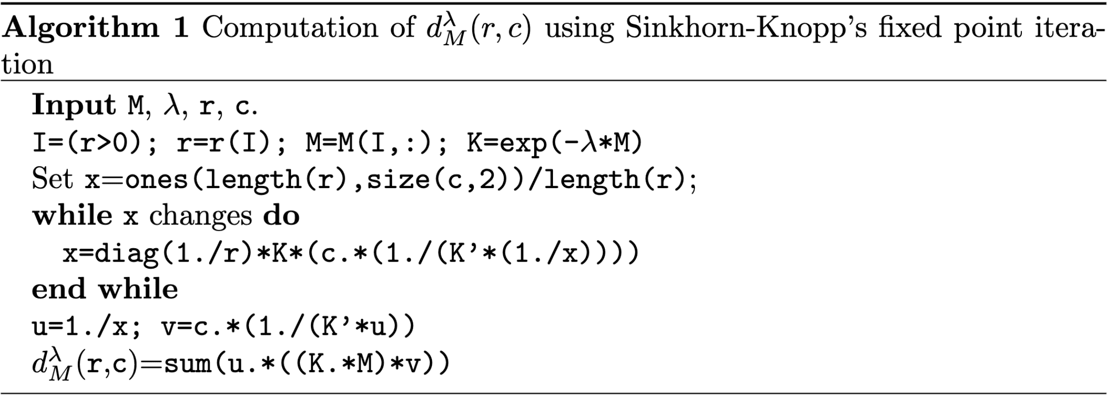
It can be readily demonstrated that the optimum of the transportation problem $d_\mathbf{M} (r, c) = \min_{\mathbf{P} \in U(r, c)} \langle \mathbf{P}, \mathbf{M} \rangle $ is a distance whenever $\mathbf{M}$ is itself a metric matrix, namely whenever $\mathbf{M}$ belongs to
\[\mathcal{M}=\left\{\mathbf{M} \in \mathbb{R}_{+}^{d \times d}: \forall i \leq d, \mathbf{M}_{i i}=0 ; \forall i, j, k \leq d, \mathbf{M}_{i j} \leq \mathbf{M}_{i k}+\mathbf{M}_{k j}\right\}\]Upon this mathematical fact, Cuturi et al. defines the Sinkhorn distance $d_{\mathbf{M}, \alpha} (r, c)$ as the optimum of a revised optimal transportation problem with an entropic regularization term:
\[d_{\mathbf{M}, \alpha} (r, c) = \underset{\mathbf{P} \in U_{\alpha} (r,c)}{\min} \langle \mathbf{P}, \mathbf{M} \rangle \\ \begin{aligned} \text{ where } U_{\alpha} (r,c) & = \{ \mathbf{P} \in U (r, c) \mid \textrm{KL}(\mathbf{P} \| rc^\top ) \leq \alpha \} \\ & = \{ \mathbf{P} \in U (r, c) \mid \mathbb{H}(\mathbf{P}) \geq \mathbb{H}(r) + \mathbb{H}(c) − \alpha \} \end{aligned}\]Note that $rc^\top$ can be construed as a probability distribution that induces the transportation plan; if a supply point possesses more, it should accordingly transport more, while for the demand point, if it demands more, it should receive proportionally more from each supply point. This constraint aims to smooth the classical optimal transportation problem, rendering the resulting optimum to be computed much faster than usual transportation solvers. In vision applications like color transfer, it is also reported by prior works that an optimal matching may lack regularity, but this issue can be addressed by applying appropriate relaxation and penalization techniques to the transportation problem.
To relief the non-convexity of the revised problem, we define the dual-Sinkhorn divergence $d_{\mathbf{M}}^\lambda$ of the same program but with a Lagrange multiplier for the entropy constraint:
\[d_{\mathbf{M}}^\lambda(r, c) = \left\langle \mathbf{P}^\lambda, \mathbf{M} \right\rangle, \text { where } \mathbf{P}^\lambda=\underset{\mathbf{P} \in U(r, c)}{\operatorname{arg min }} \left[ \langle \mathbf{P}, \mathbf{M} \rangle-\frac{1}{\lambda} \mathbb{H}(\mathbf{P}) \right]\]By duality theory we have that for every pair $(r, c)$, to each $\alpha$ corresponds an $\lambda \in [0, \infty]$ such that $d_{\mathbf{M},\alpha} (r,c) = d_{\mathbf{M}}^\lambda (r, c)$. By Lagrange multiplier method, it is equivalent to introduce the following auxiliary function:
\[\mathcal{L} = \sum_{i, j} \mathbf{P}_{ij} \mathbf{M}_{ij} - \frac{1}{\lambda} \mathbb{H} (\mathbf{P}) + \boldsymbol{\alpha}^\top (\mathbf{P} \mathbf{1} − r) + \boldsymbol{\beta}^\top (\mathbf{P}^\top \mathbf{1} − c) = 0\]where $\boldsymbol{\alpha}$ and $\boldsymbol{\beta}$ are Lagrange multipliers, and solve the following equation:
\[\frac{\partial \mathcal{L}}{\partial \mathbf{P}_{ij}} = \mathbf{M}_{ij} + \frac{1}{\lambda} \log \mathbf{P}_{ij} + \frac{1}{\lambda} + \boldsymbol{\alpha}_i + \boldsymbol{\beta}_j = 0\]Then, we obtain
\[\mathbf{P}_{ij} = e^{-\lambda \boldsymbol{\alpha}_i - 0.5} e^{-\lambda \mathbf{M}_{ij}} e^{-\lambda \boldsymbol{\beta}_j - 0.5}\]Hence, it suffices to find two vectors $\boldsymbol{\alpha} > 0$ and $\boldsymbol{\beta} > 0$ such that
\[\mathbf{P} = \textrm{diag}(\boldsymbol{\alpha}) e^{-\lambda \mathbf{M}} \textrm{diag}(\boldsymbol{\beta})\]The existence & uniqueness (up to scalar multiplication) of the solution of the problem are well known by the following theorem, called Sinkhorn’s theorem:
If a square matrix $A \in \mathbb{R}^{n \times n}$ is a matrix with strictly positive elements, there exist diagonal matrices $D_1$ and $D_2$ with strictly positive diagonal elements such that $D_1 A D_2$ is doubly stochastic, i.e. each column sum and row sum is $1$. The matrices $D_1$ and $D_2$ are unique modulo multiplying the first matrix by a positive number and dividing the second one by the same number.
Given $e^{−\lambda \mathbf{M}}$ and marginals $r$ and $c$, it is thus sufficient to run enough iterations of Sinkhorn-Knopp’s algorithm to converge to a solution $\mathbf{P}^\lambda$ of that problem.
Leave a comment