[Representation Learning] CLIP

Traditional computer vision models have predominantly enhanced their performance by exclusively learning from crowd-labeled image datasets such as ImageNet. However, such an approach shows the limited robustness and generalization, for example in zero-shot setting. Simultaneously, language models have undergone rapid development with vast web-scale language datasets rather than crowd-labeled NLP datasets, surpassing the flexibility of vision models. The question then arises: Could scalable pre-training methods which learn directly from web text result in a similar breakthrough in computer vision?

In light of this, the authors of Radford et al. 2021 posited that adopting the approach of learning from large scale web text datasets could significantly contribute to the realm of image recognition. And this concept introduces a novel perspective to pre-training methodologies of vision model termed CLIP; Contrastive Language-Image Pre-training that leverages natural language supervision.

Constrastive Learning with Natural Language Supervision

Learning from natural language is a difficult task due to the wide variety of descriptions, comments, and related text that co-occur with images. Furthermore, the authors initially attempted to jointly train the vision model and text transformer, but it has limited scalability and poor computational efficiency.

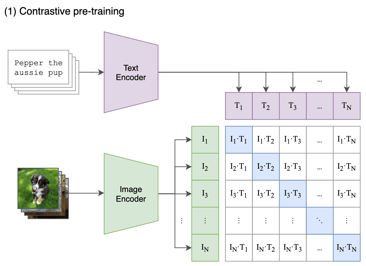
Upon the success of constrastive learning for representation learning, CLIP leverages the constrastive objective to design the potentially easier proxy task of predicting only which text as a whole is paired with which image, not the exact words of that text. Given a batch of $N$ (image, text) pairs, CLIP is trained to predict which of $N \times N$ possible (image, text) pairings across a batch actually occurred.

$\mathbf{Fig\ 1.}$ Constrastive pre-training of CLIP (Radford et al. 2021)

1. Extract feature representation of each modality
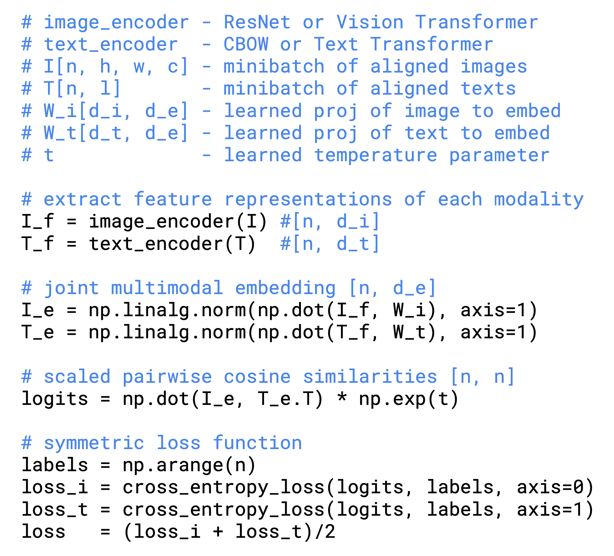
   Given image batch $I \in \mathbb{R}^{N \times H \times W \times C}$ and text batch $T \in \mathbb{R}^{N \times \ell}$, extract the feature representations with image and text encoder $f_I \in \mathbb{R}^{N \times d_i}$ and $f_T \in \mathbb{R}^{N \times d_t}$: $$ \begin{aligned} I_f = f_I (I), T_f = f_T (T) \end{aligned} $$ In the paper, it employed ResNet and ViT for $f_I$, and Transformer for $f_T$. Also, transformation operation of text and image, $t_u$ and $t_v$ as SimCLR are removed or simplified. Only random square crop of image is the only data augmentation used during training.
2. Projection to multi-modal embedding space
   Instead of non-linear projection head in SimCLR, CLIP adopts a linear projection $W_i \in \mathbb{R}^{d_i \times d_e}$ and $W_t \in \mathbb{R}^{d_t \times d_e}$ to map from each encoder representation $I_f, T_f$ to the multi-modal embedding space, $I_e, T_e \in \mathbb{R}^{N \times d_e}$. $$ \begin{aligned} I_e = \frac{I_f W_i}{\lVert I_f W_i \rVert}, T_e = \frac{T_f W_t}{\lVert T_f W_t \rVert} \end{aligned} $$
3. Learn the embedding space
   CLIP jointly trains an image and text encoder to maximize the cosine similarity of the image and text embeddings of the $N$ positive pairs in the batch while minimizing the cosine similarity of the embeddings of the $N^2 − N$ negative pairings. To do so, it optimizes a symmetric cross entropy loss over these similarity scores. Each cross entropy loss of cosine similarity is also known as multi-class N-pair loss. $$ \begin{aligned} \mathcal{L}_{\mathrm{total}} & = (\mathcal{L}_{\mathrm{image}} + \mathcal{L}_{\mathrm{text}}) / 2 \\ \mathcal{L}_{\mathrm{image}} & = \sum_{i=1}^N -\log \left[ \frac{\exp (\text{sim} (I_{e, i}, T_{e, i}) / \tau)}{\sum_{j = 1}^N \exp (\text{sim} (I_{e, i}, T_{e, j}) / \tau) } \right] \\ \mathcal{L}_{\mathrm{text}} & = \sum_{i=1}^N -\log \left[ \frac{\exp (\text{sim}(I_{e, i}, T_{e, i}) / \tau) }{\sum_{j = 1}^N \exp (\text{sim}(I_{e, j}, T_{e, i}) / \tau) } \right] \end{aligned} $$ where $\tau$ is learned temperature parameter and $\text{sim} (\boldsymbol{u}, \boldsymbol{v}) = \boldsymbol{u}^\top \boldsymbol{v} / \lVert \boldsymbol{u} \rVert \lVert \boldsymbol{v} \rVert$. In PyTorch, each cross entropy loss can be implemented as nn.CrossEntropyLoss(logits_per_image/text, torch.arange(N)).

The numpy-style pseudocode of training CLIP is outlined in $\mathbf{Fig\ 2}$.

$\mathbf{Fig\ 2.}$ Constrastive pre-training of CLIP (Radford et al. 2021)

Zero-Shot Transfer

To leverage CLIP for zero-shot classification, the image encoder computes a feature representation for the image, and the text encoder acts as a hypernetwork (a network that generates the weights for another network) that generates the weights of linear classifier based on the text specifying the visual concepts that the classes represent. In detail, it first computes the feature embedding of the image and that of the set of possible texts (e.g. class names). The cosine similarity of these embeddings is then calculated, scaled by a temporature $\tau$, and normalized via softmax.

$\mathbf{Fig\ 3.}$ CLIP Classifier (Radford et al. 2021)

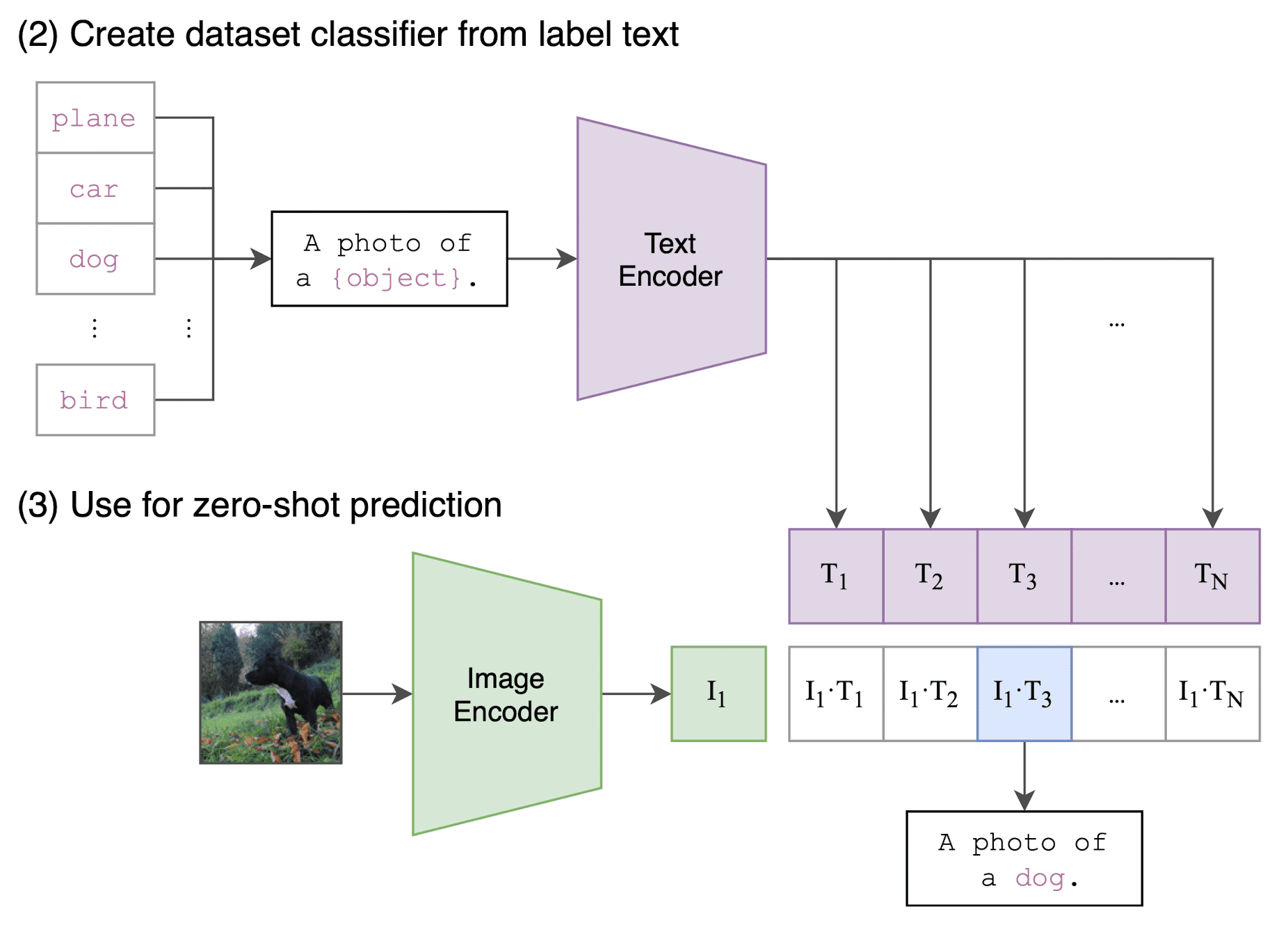
The critical things here are polysemy in texts and distribution gap. When solely presented with the name of a class, CLIP’s text encoder faces difficulty in differentiating the intended word sense due to the lack of context. For instance, in ImageNet, the term “crane” could refer to both construction cranes and flying cranes. Another instance is found in the Oxford-IIIT Pet dataset, where the term “boxer” contextually signifies a breed of dog, but to a text encoder devoid of context, it could just as easily be interpreted as a type of athlete. Also, within the pre-training dataset of CLIP, it’s relatively rare for the text paired with the image to be just a single word, but it is typically a full sentence.

These issues are possible to be mitigated by prompt engineering. For example, the authors found that “A photo of a {label}.” is a good default that helps specify the text is about the content of the image, improving performance. (+1.3% for ImageNet) Also, they found that dataset-specific prompt text can significantly improve the performance. Here are some examples.

• Oxford-IIIT Pets
  • “A photo of a {label}, a type of pet.”
• Satellite image classification datasets
  • “a satellite photo of a {label}.”

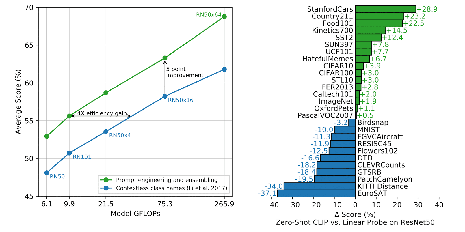
Moreover, the paper experimented that ensembling over multiple zero-shot classifiers, using different context prompts such as “A photo of a big {label}” and “A photo of a small {label}”, can help improving performance. To maintain the computing cost of a single classifier, they construct the ensemble over the embedding space instead of probability space.

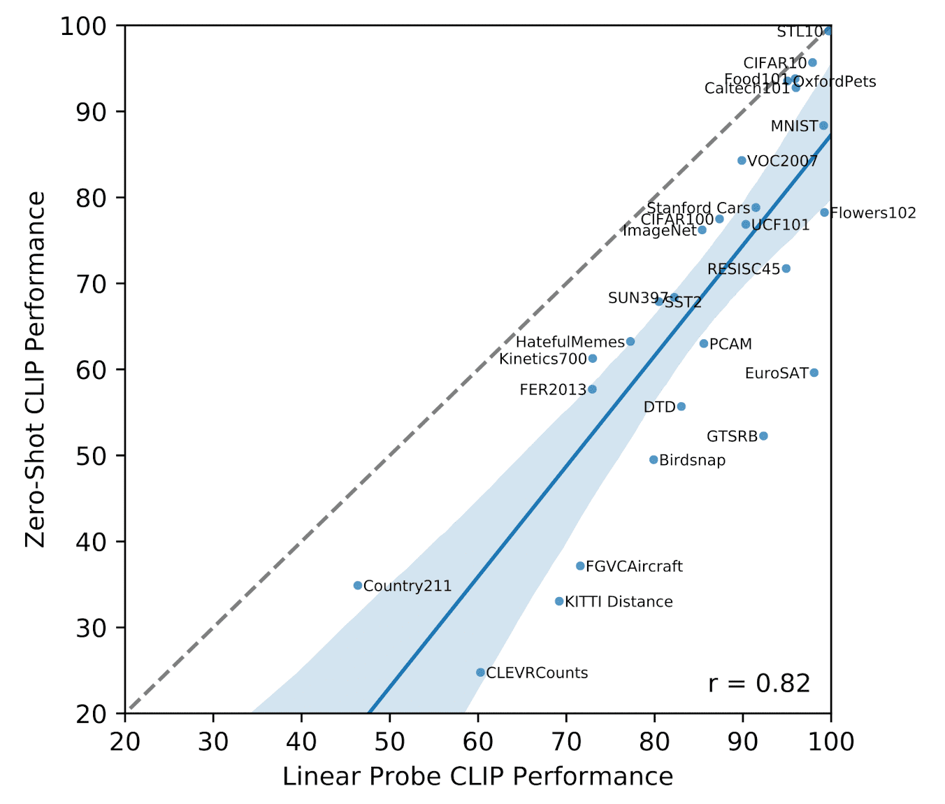
As a result, zero-shot CLIP outperforms a fully supervised linear classifier fitted on ResNet-50 feature (linear probing), on 16 of the 27 datasets. (See $\mathbf{Fig\ 4.}$) Looking at where zero-shot CLIP notably underperforms, zero-shot CLIP is quite weak on several fine-grained, specialized, complex, or abstract tasks:

• satellite image classification
  • EuroSAT, RESISC45
• lymph node tumor detection
  • PatchCamelyon
• counting objects in synthetic scenes
  • CLEVRCounts
• self-driving related tasks
  • GTSRB, KITTI Distance

$\mathbf{Fig\ 4.}$ (Left) Power of prompt engineering and ensembling (Right) Zero-shot CLIP is competitive with a fully supervised baseline (Radford et al. 2021)

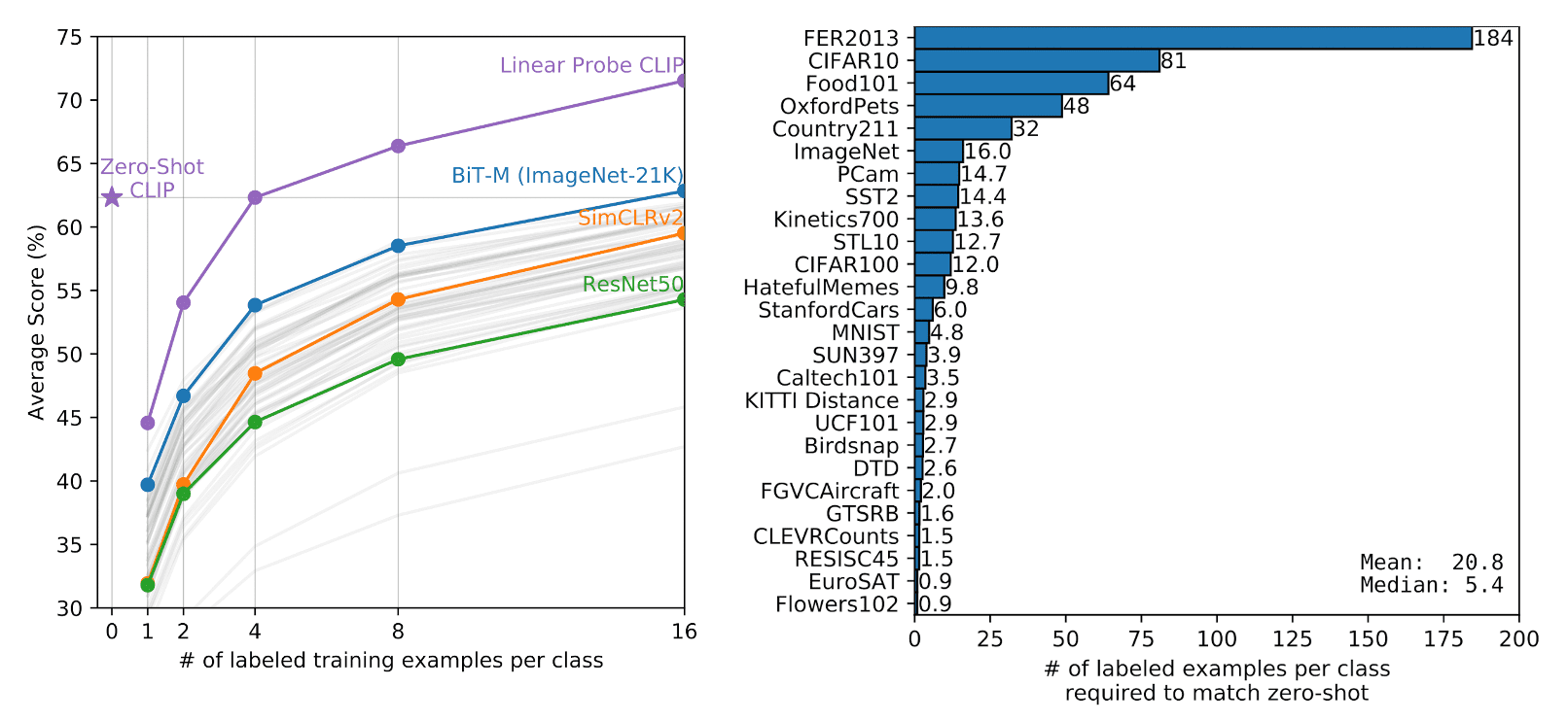
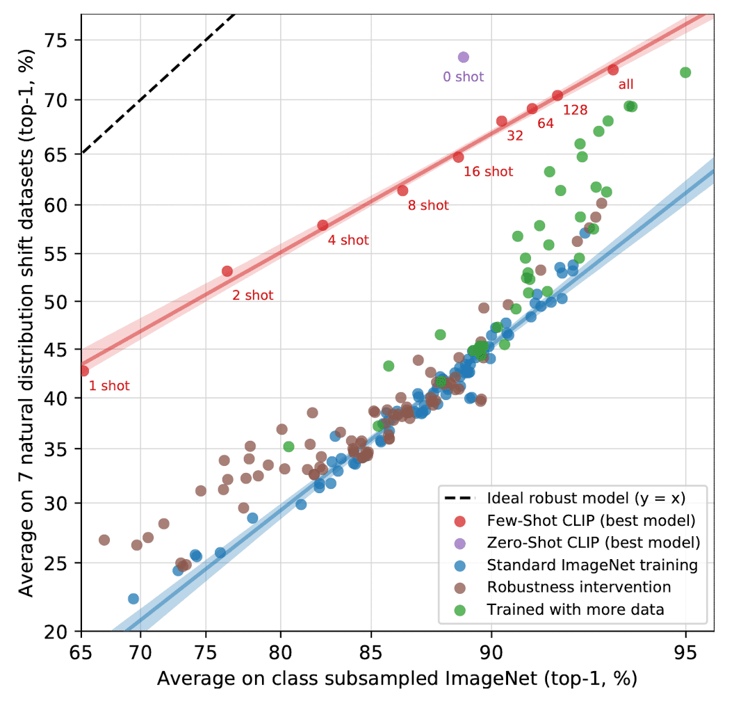
Next, the paper compares zero-show CLIP with few-shot linear probes, including linear probe CLIP. (See $\mathbf{Fig\ 5.}$) Surprisingly, zero-shot CLIP matches the performance of the best performing 16-shot classifier in the evaluation suite, and 4-shot logistic regression on the same feature space of CLIP. This discrepancy primarily arises from a significant distinction between the zero-shot and few-shot approaches. CLIP’s zero-shot classifier is formulated through natural language, enabling direct specification (communication) of visual concepts. In contrast, normal supervised learning must deduce concepts indirectly from training examples.

$\mathbf{Fig\ 5.}$ (Left) Comparison with few-shot linear probes (Right) The data efficiency of zero-shot transfer (Radford et al. 2021)

And $\mathbf{Fig\ 6.}$ illustrates CLIP’s zero-shot performance in comparison to fully supervised linear classifiers across datasets. Across most datasets, zero-shot classifiers exhibit a performance gap of 10% to 25% when compared to fully supervised classifiers, indicating room for enhancement in CLIP’s task-learning and zero-shot transfer capabilities. Notably, zero-shot CLIP only approaches fully supervised performance on 5 datasets (STL10, CIFAR10, Food101, OxfordPets, and Caltech101). This suggests that CLIP may be more effective at zero-shot transfer for tasks where its underlying representations are of high quality.

$\mathbf{Fig\ 6.}$ Comparison with fully supervised classifiers (Radford et al. 2021)

Experiments

Representation Learning

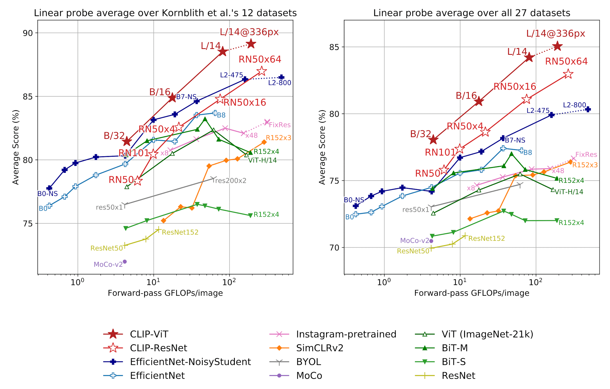
Following the evaluation convention in the field of representation learning, the paper also explored fine-tuning and linear probing performance of CLIP to evaluate the representation quality of CLIP. For fair evaluation of the quality of learned CLIP representation, the paper opts for linear probing and $\mathbf{Fig\ 7.}$ shows the result. All CLIP models outperform all evaluated systems in terms of compute efficiency.

$\mathbf{Fig\ 7.}$ Linear probe performance of CLIP in comparison with SOTA computer vision models (Radford et al. 2021)

Robustness to natural distribution shift

To discuss the robustness of CLIP, we should define what the robustness does exactly mean. Taori et al. 2020 distinguishes the robustness in two categories:

• Effective robustness: measurements of improvements in accuracy under distribution shift
• Relative robustness: measurements of improvements in out-of-distribution accuracy

And they argue that robustness techniques should aim to improve both effective robustness and relative robustness. In order to evaluate the robustness of CLIP, the paper compare the performance of zero-shot CLIP that is not able to exploit dataset-specific correlations or patterns, with existing ImageNet models on natural distribution shifts ¹. See $\mathbf{Fig\ 8.}$ for the result. An ideal robust model (dashed line) should performsequally well on the ImageNet distribution and on other natural image distributions (ImageNet V1, ImageNet V2, ImageNet-R, ObjectNet, ImageNet Sketch, ImageNet-A).

$\mathbf{Fig\ 8.}$ Robustness of zero-shot CLIP compared to the standard ImageNet model (Radford et al. 2021)

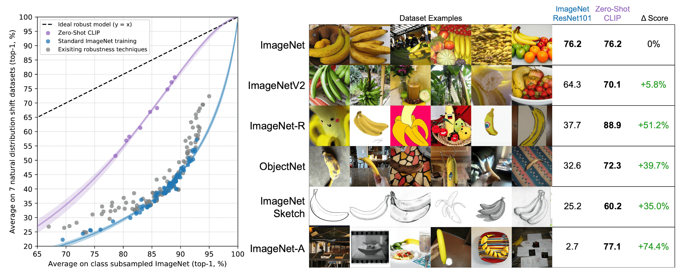
In addition, the next experiment demonstrates that supervised learning on ImageNet doesn’t necessarily cause a robustness gap, by showing that CLIP could also result in much more robust models regardless of whether they are zero-shot or fine-tuned. $\mathbf{Fig\ 9.}$ illustrates the performance change after adapting to the ImageNet distribution via a $L_2$ regularized logistic regression classifier fit to CLIP features on the ImageNet training set.

$\mathbf{Fig\ 9.}$ Performance change while supervised adaptation (Radford et al. 2021)

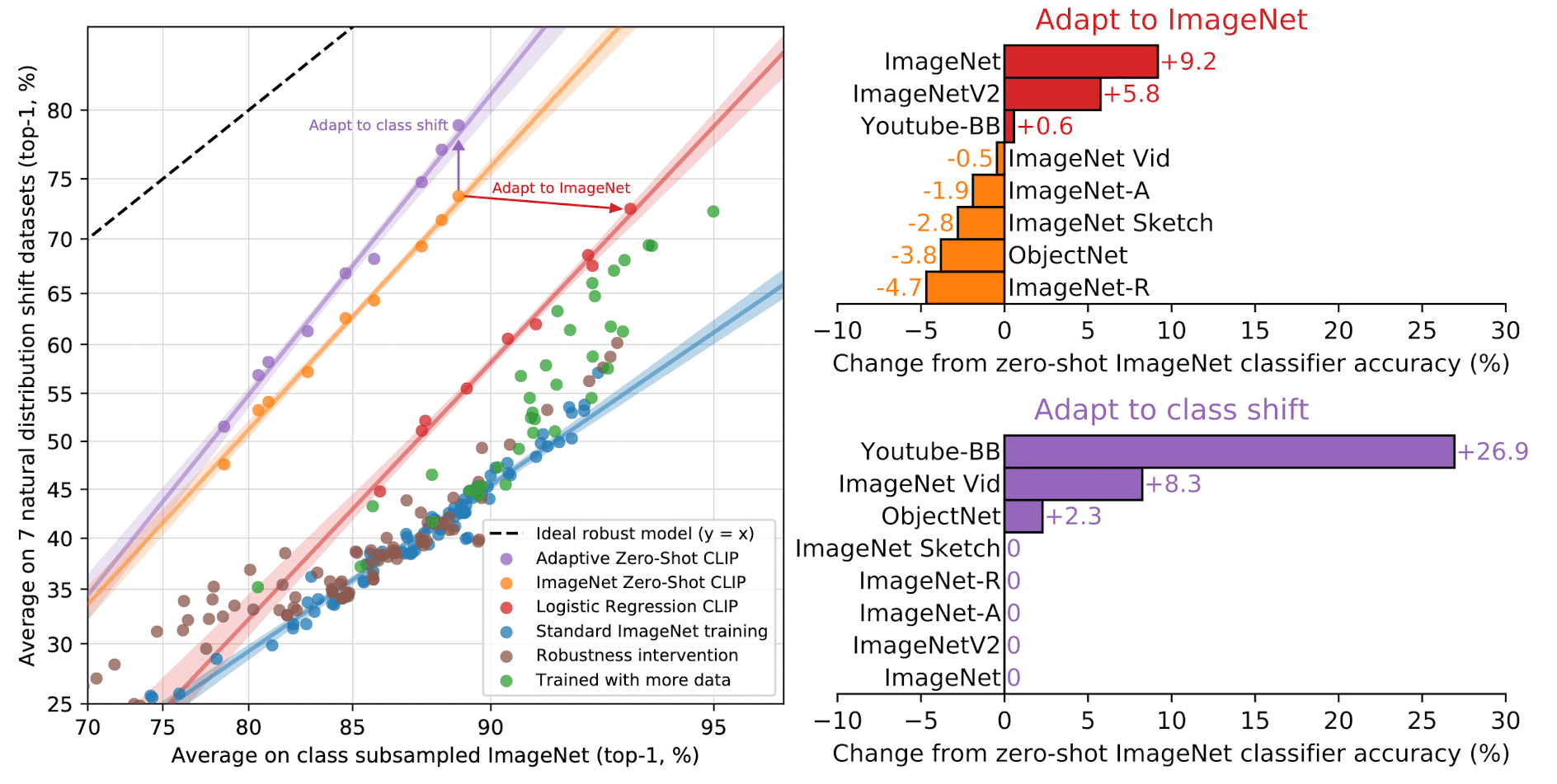
$\mathbf{Fig\ 10.}$ depicts how effective robustness changes across the continuum from zero-shot to fully supervised. It is evident that few-shot models exhibit increased effective robustness compared to existing models, but this robustness diminishes as in-distribution performance improves with more training data, and is largely absent for the fully supervised model. Furthermore, zero-shot CLIP demonstrates noteworthy robustness, surpassing that of a few-shot model with equivalent ImageNet performance.

$\mathbf{Fig\ 10.}$ Few-shot CLIP also increases effective robustness (Radford et al. 2021)

Limitations

• The supervised baseline that the paper employs a linear classifier on top of ResNet models. The performance of this baseline is now well below the current SOTA. The authors estimate around a $1000x$ increase in compute is required for zero-shot CLIP to reach that.
• CLIP’s zero-shot performance is still quite weak or near random on several kinds of tasks.
  • fine-grained classification such as differentiating models of cars, species of flowers, and variants of aircraft.
  • abstract and systematic tasks such as counting the number of objects in an image.
  • novel tasks which are unlikely to be included in CLIP’s pre-training dataset, such as classifying the distance to the nearest car in a photo.
• Zero-shot CLIP still generalizes poorly to data that is truly out-of-distribution for it. For example, CLIP learns the high quality of OCR representation, it only achieves 88% accuracy on of MNIST (less than simple logistic regression).
• CLIP does not address the poor data efficiency of deep learning. Instead, it mitigates this limitation by leveraging a scalable source of supervision, encompassing hundreds of millions of training examples. If each image encountered during the training of a CLIP model was presented at a rate of one per second, it would take 405 years to iterate through the 12.8 billion images observed over 32 training epochs.

Footnotes

1. Taori et al. 2020 distinguishes between natural distribution shifts and synthetic distribution shifts, based on the source of distribution shift. The datasets such as ImageNet-C, Stylized ImageNet, or adversarial attacks have synthetic distribution shifts since they are created by perturbing existing images in various ways. The reason of this distinction is because they found that while several techniques have been demonstrated to improve performance on synthetic distribution shifts, they often fail to yield consistent improvements on natural distributions.

Reference

[1] Radford et al. “Learning Transferable Visual Models from Natural Language Supervision.” International Conference on Machine Learning. PMLR, 2021.
[2] OpenAI Blog, “CLIP: Connecting text and images”, 2021/01/05
[3] Taori et al. “Measuring robustness to natural distribution shifts in image classification.” NeurIPS 2020