[Representation Learning] Masked Image Modeling (MIM)

Introduction

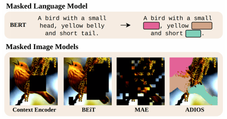
Contrastive learning techniques have become the dominant visual pre-training framework since the advent of contrastive self-supervised learning in 2018. Starting from BEiT, however, this framework has been challenged by a generative technique called masked image modeling (MIM), a mask prediction strategy that trains the model using target visual tokens generated by an off-the-shelf tokenizer. The success of masked image modeling in vision opens the door to a trajectory similar to that of NLP for self-supervised learning in vision.

$\mathbf{Fig\ 1.}$ Masked Image Modeling (OpenMixup)

BERT Pre-Training of Image Transformers (BEiT)

Motivated by the unprecedented success of BERT in NLP, Bao et al., 2022 proposed vision-style BERT training termed BEiT, which randomly masks image patches and trains to recover the visual tokens of masked patches (instead of the raw pixels).

Similar to ViT, the 2D input image is split into a grid of patches. Since the pixel-level recovery task tends to waste modeling capability on pre-training short-range dependencies and high-frequency details, patches are tokenized to discrete visual tokens. Then, a proportion of image patches are randomly masked, and the model learns to recover the visual tokens of the original image from the corrupted input.

$\mathbf{Fig\ 2.}$ Overview of BEiT Pre-training (Bao et al., 2022)

In particular, BEiT pre-training consists of two separated stages:

1. Learning Visual Tokens
   Similar to word embeddings in BERT, the 2D input image $\boldsymbol{x} \in \mathbb{R}^{H \times W}$ is tokenized to discrete tokens, which is modeled by the latent codes of discrete VAE (dVAE) $\boldsymbol{z} = [z_1, \cdots, z_N] \in \mathcal{V}^{N}$, where each $z_i$ is discrete token indices contained in the vocabulary $\mathcal{V} = \{1, \cdots, \vert \mathcal{V} \vert \}$.
   
   Formally, the tokenizer (encoder of dVAE) $q_\phi (\boldsymbol{z} \vert \boldsymbol{x})$ maps image pixels into a visual codebook, and the decoder $p_\psi (\boldsymbol{x} \vert \boldsymbol{z})$ learns to reconstruct the input image. The paper represent each $224 \times 224$ image into a $14 \times 14$ grid of discrete image tokens, each element of which can assume $\vert \mathcal{V} \vert = 8192$ possible values.
   

   

   $\mathbf{Fig\ 3.}$ Learning an image tokenizer (Bao et al., 2022)
   
   
2. Masked Image Modeling
   The standard ViT is used for the backbone network. The 2D input image $\boldsymbol{x} \in \mathbb{R}^{H \times W \times C}$ is split into $N = H \cdot W / P^2$ number of patches $\{ \boldsymbol{x}_i^p \in \mathbb{R}^{P \times P \times C} \}_{i=1}^N$. Some image patches are randomly masked ($\approx 40\%$) with a learnable embedding $\boldsymbol{e}_\texttt{[M]} \in \mathbb{R}^D$ where the masked positions are denoted as $\mathcal{M} \in \{1, \cdots, N\}^{0.4}$, producing the corrupted image $\boldsymbol{x}^\mathcal{M}$: $$ \boldsymbol{x}^\mathcal{M} = \{ \boldsymbol{x}_i^p \vert i \notin \mathcal{M} \}_{i=1}^N \cup \{ \boldsymbol{e}_\texttt{[M]} \in \mathbb{R}^D \vert i \in \mathcal{M} \}_{i=1}^N $$ Then, the corrupted image is processed by ViT that yields the hidden vectors $\{ \boldsymbol{h}_{i=1}^L \}_{i=1}^N = \texttt{ViT}(\boldsymbol{x}^\mathcal{M})$. Subsequently, the visual tokens that corresponds to the masked patches are predicted by a softmax classifier: $$ \mathrm{p}_{\textrm{MIM}}(z^\prime \vert \boldsymbol{x}^\mathcal{M}) = \texttt{softmax}_{z^\prime} (\boldsymbol{W}_c \boldsymbol{h}_i^L + \boldsymbol{b}_c) \text{ with } \boldsymbol{W}_c \in \mathbb{R}^{\vert \mathcal{V} \vert \times D}, \boldsymbol{b}_c \in \mathbb{R}^{\vert \mathcal{V} \vert} $$ where the objective is maximizing the log-likelihood of the ground-truth visual tokens $\boldsymbol{z}^\prime = [z_i \in \boldsymbol{z} \vert i \in \mathcal{M}]$ given the corrupted image $\boldsymbol{x}^\mathcal{M}$ with the masked positions $\mathcal{M}$: $$ \mathcal{L}_{\textrm{MIM}} = \sum_{\boldsymbol{x} \in \mathcal{D}} \mathbb{E}_\mathcal{M} \left[ \sum_{i \in \mathcal{M}} \log \mathrm{p}_{\textrm{MIM}} (z_i \vert \boldsymbol{x}^\mathcal{M}) \right] $$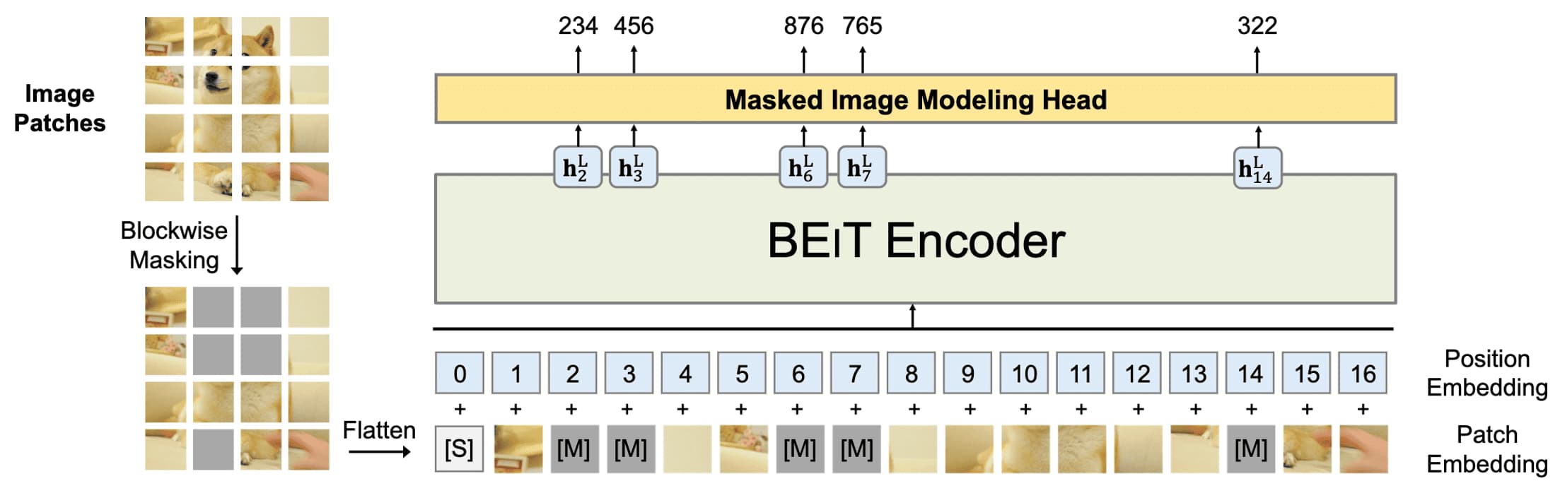

   

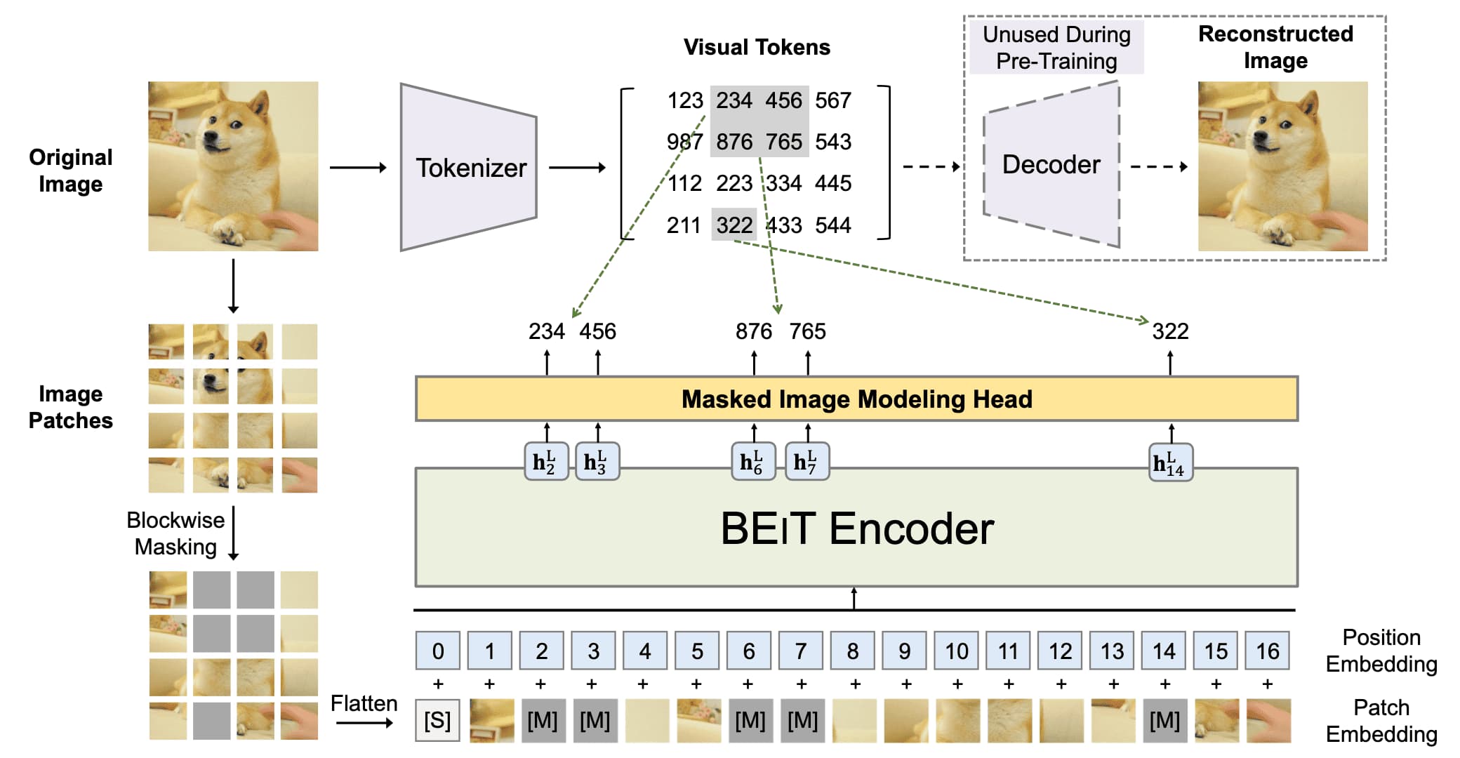
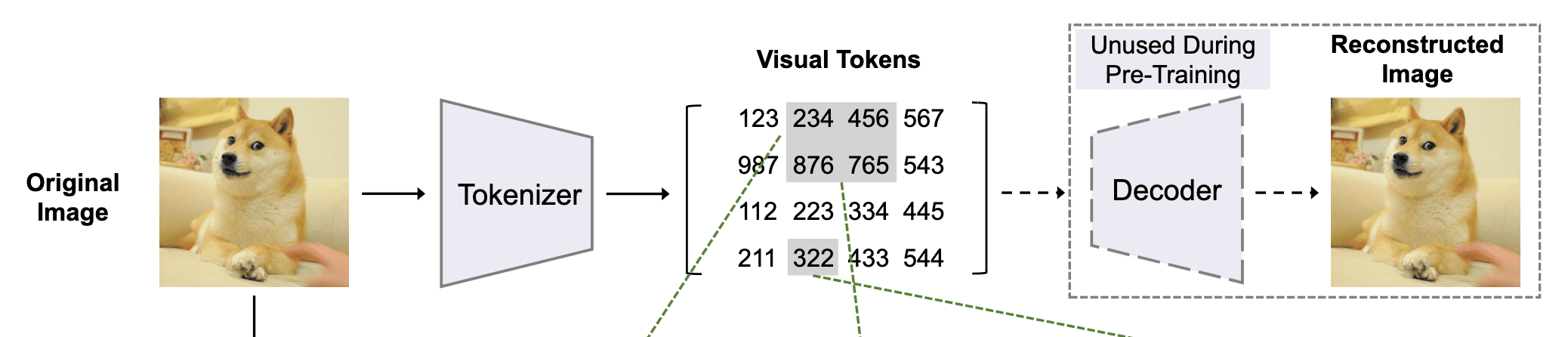
   $\mathbf{Fig\ 4.}$ Masked Image Modeling of BEiT (Bao et al., 2022)
   
   

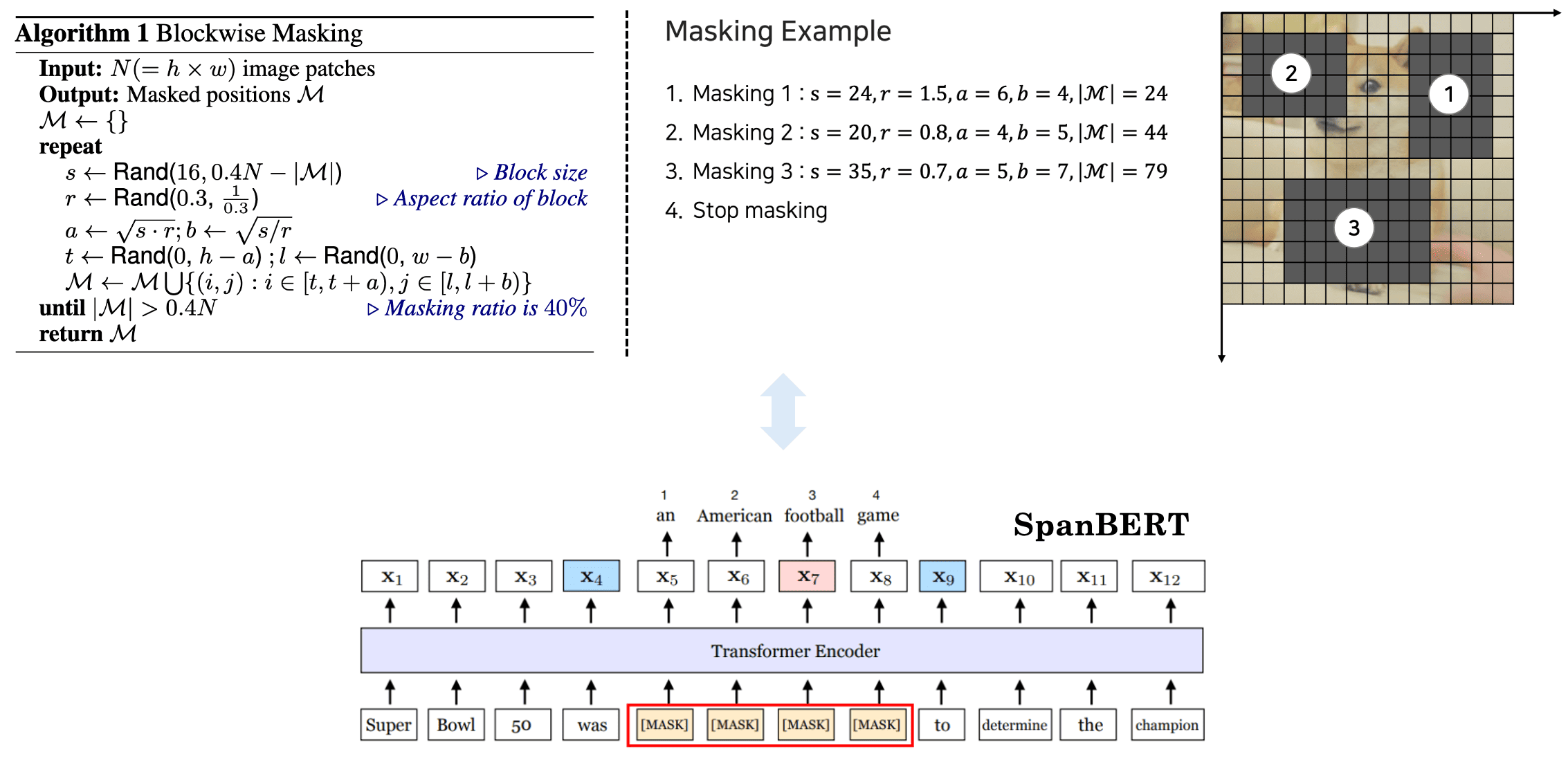
For selecting the masking position $\mathcal{M}$, motivated by SpanBERT, block-wise (N-gram) masking strategy is used. As illustrated in the figure below, a block of random resolution (with the minimum number of patches to $16$) is masked each iteration. This is repeate until obtaining enough masked patches (total $40\%$ of patches).

$\mathbf{Fig\ 5.}$ Blockwise Masking in BEiT

End-to-end Masked Auto-Encoder

The tokenizer is pretrained by a dVAE, and therefore BEiT consists of two-stage training. He et al., 2022 and Xie et al., 2022 concurrently proposed end-to-end masked auto-encoders in the vision termed masked autoencoder (MAE) and simple MIM (SimMIM), respectively, which are both accepted at CVPR 2022 and have attracted unprecedented attention.

Masked Auto-Encoder (MAE)

Contrast to BEiT that predicts discrete token of masked patches, MAE revisits the pretext task of predicting the pixel values for each masked patch. Specifically, it optimizes simple MSE loss of masked patches to directly predicts masked patches from the unmasked ones.

$\mathbf{Fig\ 6.}$ MAE: Masked Auto-Encoder (He et al., 2022)

MAE is chracterized by two key components:

1. High masking ratio
   While BERT masks $15\%$ and BEiT masks $40\%$ of tokens, MAE set higher masking ratio (e.g. $75\%$). This leads to reduction in computation of large encoder since it processes only a small portion of patches.
   
   

   

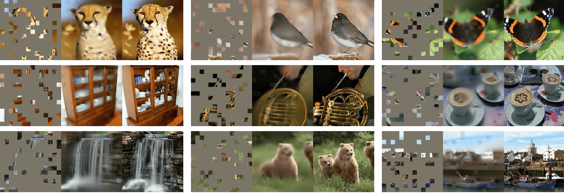
   $\mathbf{Fig\ 7.}$ Left: the masked image (with ratio of $80\%$), Mid: MAE reconstruction, Right: ground-truth. (He et al., 2022)
   
   Furthermore, a high masking ratio can also improve accuracy; ablation findings support that such a high masking ratio is beneficial for both fine-tuning and linear probing. This also motivates recent work to experiment in masked language modeling with a higher masking rate for greater effectiveness.
   
   

   

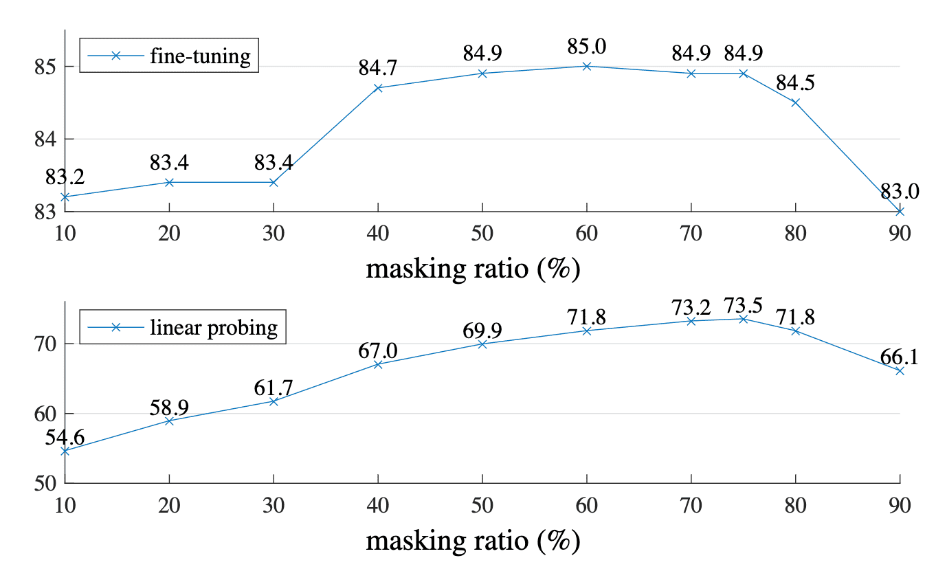
   $\mathbf{Fig\ 8.}$ A high masking ratio ($75\%$) works well for both fine-tuning and linear probing. (He et al., 2022)
   
   
2. Asymmetric encoder-decoder architecture
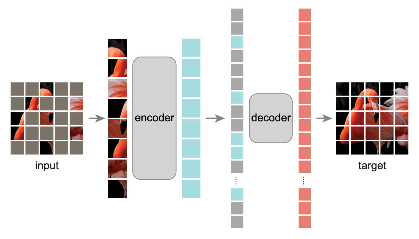
   MAE designs an asymmetric encoder-decoder architecture with lightweight decoder, enabling the training of a large ViT encoder. Additionally, the encoder of MAE operates only on the unmasked patches, so the combination of the asymmetric architecture and higher masking ratio significantly reduces the pre-training time (MAE is $3\times$ or more faster than BEiT, while achieving superior performance).
   
   In the paper, MAE decoder uses the decoder with $8$ blocks and a width of $512$ dim, which has $9\%$ FLOPs per token vs. ViT-L. They found that the decoder depth is less influential for improving fine-tuning, and only a single transformer block decoder can perform strongly with fine-tuning.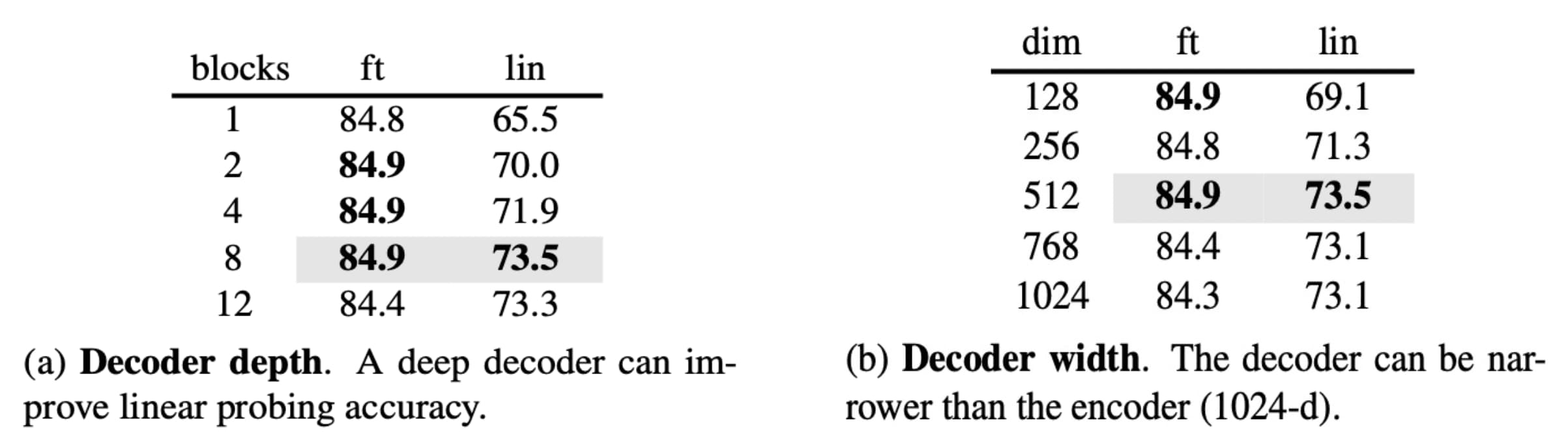

   

   $\mathbf{Fig\ 9.}$ Masked Image Modeling of BEiT (He et al., 2022)
   
   

In the ablation, other intriguing properties are observed:

3. Mask token
   MAE skip the mask token $\texttt{[M]}$ in the encoder and apply it later in the lightweight decoder. It is more accurate and decreases the computation time.
4. Reconstruction target
   Predicting pixels with per-patch normalization improves accuracy, which is much simpler and efficient than tokenization.
5. Data augmentation
   MAE works well using cropping-only augmentation. Interestingly, it behaves decently even if using no data augmentation.
6. Mask sampling
   Random patch masking is better than block-wise and grid-wise sampling:
   • Block-wise sampling: Removes large random blocks;
   • Grid-wise sampling: Keeps one of every four patches;

$\mathbf{Fig\ 10.}$ Properties of MAE (He et al., 2022)

Simple MIM (SimMIM)

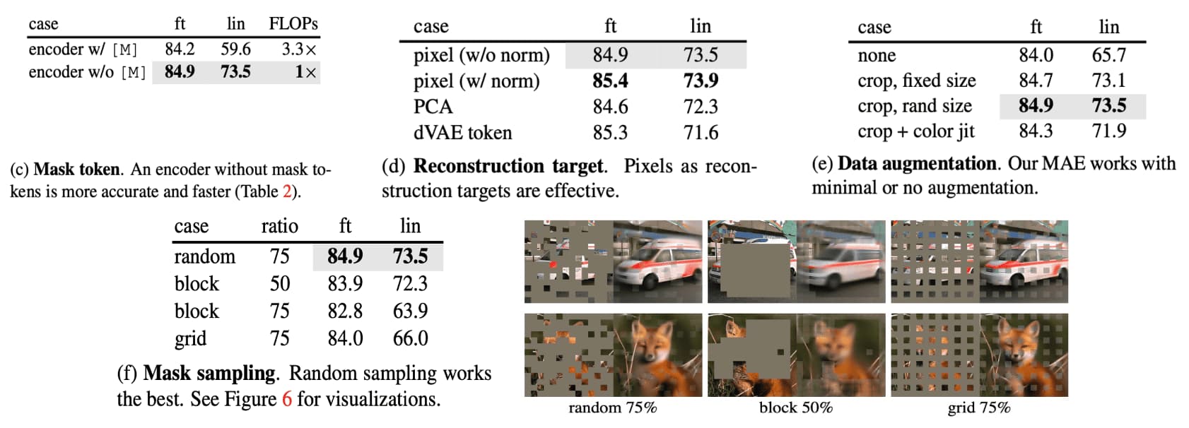
Similar to MAE, SimMIM regresses the raw pixel values of randomly masked patches using $\ell_1$ loss, demonstrating that direct pixel regression aligns well with the continuous nature of visual signals (e.g., ordering property) and performs at least as well as classification designs, such as tokenization, clustering, or discretization. SimMIM also employs a lightweight prediction head, such as a linear layer, which effectively attains comparable or slightly better performance to that of more complex prediction heads.

$\mathbf{Fig\ 11.}$ SimMIM: Simple MIM (Zhou et al., 2022)

The SimMIM framework consists of 3 major components for masked image modeling:

1. Masking Strategy
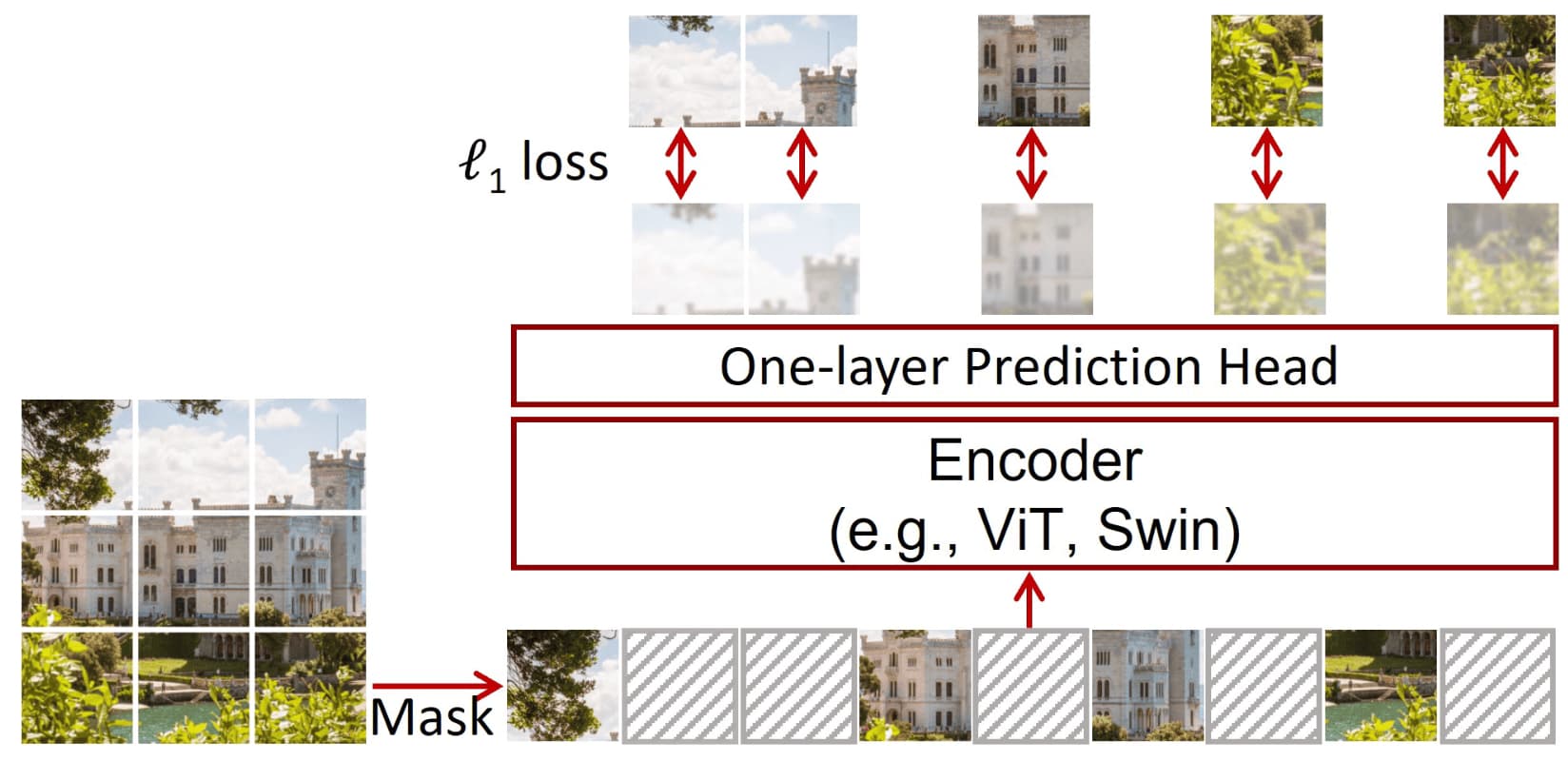
   SimSIM investigates multiple masking strategies, such as square, block-wise, and random. Their best performance is achieved with the random masking strategy, which is the same as that in MAE.
   
   

   

   $\mathbf{Fig\ 12.}$ Different masking strategies (Xie et al., 2022)
   
   Moreover, the authors discovered that a large masked patch size of $32$ is advantageous for a more robust pretext task and resilient to the masking ratio. This is because the central pixel of a large masked patch is sufficiently distant from visible pixels, compelling the network to learn relatively long-range connections, even with a low masking ratio or when surrounding patches are unmasked. For a relatively small patch size, a high masking ratio can achieve a similar effect and has also been confirmed to enhance performance.
   
   

   

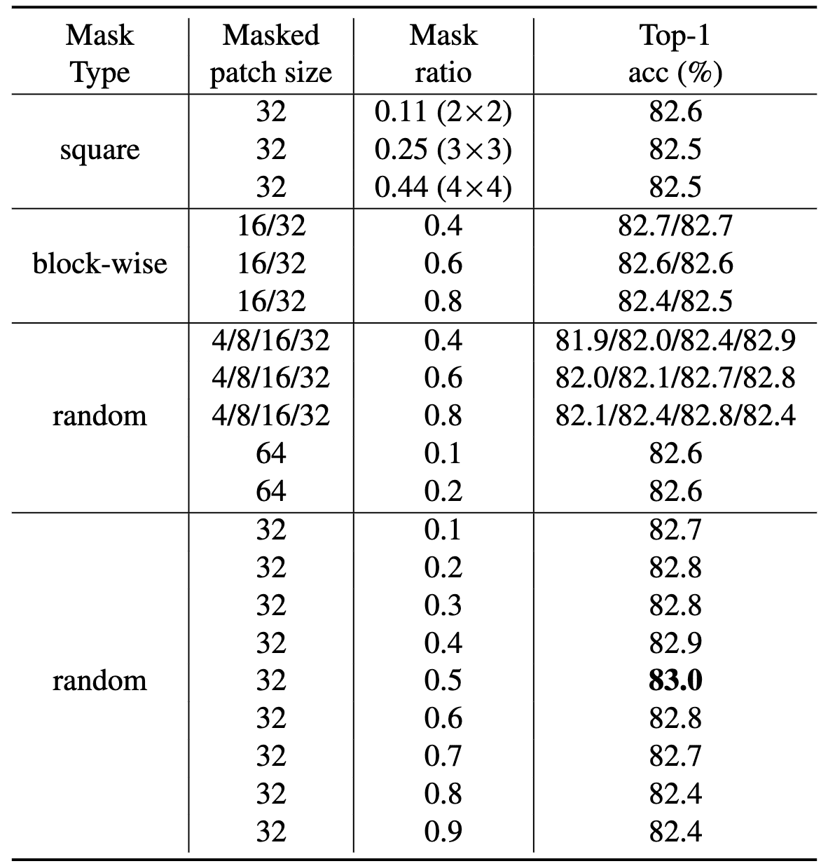
   $\mathbf{Fig\ 13.}$ Ablation on different masking strategies with different masked patch sizes (Xie et al., 2022)
   
   
2. Prediction head
   SimMIM demonstrated that the prediction head can be extremely lightweight, even as light as a linear layer, similar to MAE. Although heavier heads generally offer greater generation capability, this increased capability does not necessarily benefit downstream fine-tuning tasks. This is likely because the capacity is largely wasted in the prediction head, which is not utilized in downstream tasks.
   
   

   

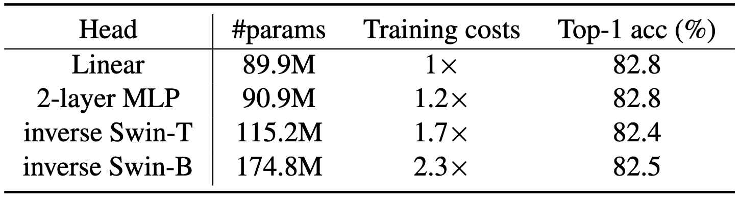
   $\mathbf{Fig\ 14.}$ Ablation on different prediction heads (Xie et al., 2022)
   
   
3. Prediction target
   The prediction head maps feature vectors from the encoder to the original resolution with output dimension $3 \times H \times W$. An $\ell_1$ loss is employed for the objective: $$ \mathcal{L} = \frac{1}{\Omega (\boldsymbol{x}_\mathcal{M})} \Vert \boldsymbol{y}_\mathcal{M} - \boldsymbol{x}_\mathcal{M} \Vert_1 $$ where $\boldsymbol{x}, \boldsymbol{y} \in \mathbb{R}^{3HW \times 1}$ are the input RGB values and the predicted values, respectively; $\mathcal{M}$ denotes the set of masked pixels; $\Omega (\cdot)$ is the number of elements.
   
   Several observations can be drawn from the ablation study:
   • The approach predicting the masked area performs significantly better than that recovering all image pixels;
   • Simple raw-pixel regression performs no worse than classification approaches with specially defined classes through tokenization, clustering, or discretization;
   • The three losses, $\ell_1$, smooth-$\ell_1$, and $\ell_2$, perform similarly well;

   

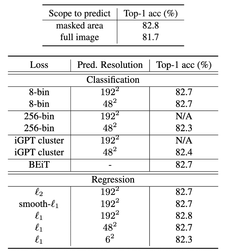
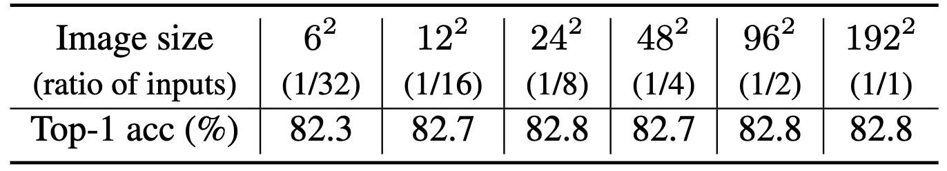
   $\mathbf{Fig\ 15.}$ Ablation on different prediction targets (Xie et al., 2022)
   
   

Interestingly, a broad range of target resolutions (e.g., $12^2$ to $96^2$) perform competitively with the highest resolution of $192^2$. The transfer performance only drops significantly at a low resolution of $6^2$, likely due to excessive information loss. These results suggest the level of information granularity required for downstream image classification tasks.

$\mathbf{Fig\ 16.}$ Ablation on different prediction resolution (Xie et al., 2022)

Difference between MAE and SimMIM

One of the differences between two methods lies in the placement of masked patch tokens:

• MAE: input of decoder
• SimMIM: input of encoder

With the pretext task of masked prediction, MAE and SimMIM carry out two roles: representation encoding for unmasked patches and pretext prediction for masked patches. In SimMIM, the encoder handles both representation encoding and pretext prediction simultaneously, unburdening the decoder to be as simple as a single layer. In contrast, MAE’s encoder only performs representation encoding, delegating pretext prediction to the decoder.

As a result, MAE still requires transformer blocks for the decoder, though it need not be as complex as the encoder. This design enables MAE to achieve significantly higher linear probing accuracy than SimMIM, which is less dependent on the projection head. However, this advantage diminishes with fine-tuning. For instance, with ViT-B as the backbone on ImageNet, SimMIM achieves a fine-tuning performance of $83.8\%$, slightly higher than the reported $83.6\%$ for MAE.

Another advantage of MAE, by feeding only the unmasked patches into the encoder, is its higher efficiency, especially with a high masking ratio. However, this makes MAE incompatible with other ViT architectures such as Swin Transformer. Several future works aim to address these issues.

Decoder-free MIM

Beyond masked autoencoder, decoder-free MIM can be viewed as another approach to simplifying BEiT, reducing it from BEiT’s two-stage stages to a single stage.

Image-BERT Pre-Training with Online Tokenizer (IBOT)

By formulating the MIM as knowledge distillation, image-BERT pre-training with online tokenizer (IBOT) discard the decoder and perform patch-level self-distillation on masked patch tokens (while DINO is done with image-level objective). Like BEiT, IBOT utilizes the image tokenizer $f_t$ for the target network $f_s$ where both share the same architecture and $f_t$ is an EMA version of $f_s$ from past iterations. However, unlike BEiT, image tokenizer is jointly learned, i.e., $f_t$ is an online tokenizer.

$\mathbf{Fig\ 17.}$ IBOT: Image-BERT Pre-Training with Online Tokenizer (Zhou et al., 2022)

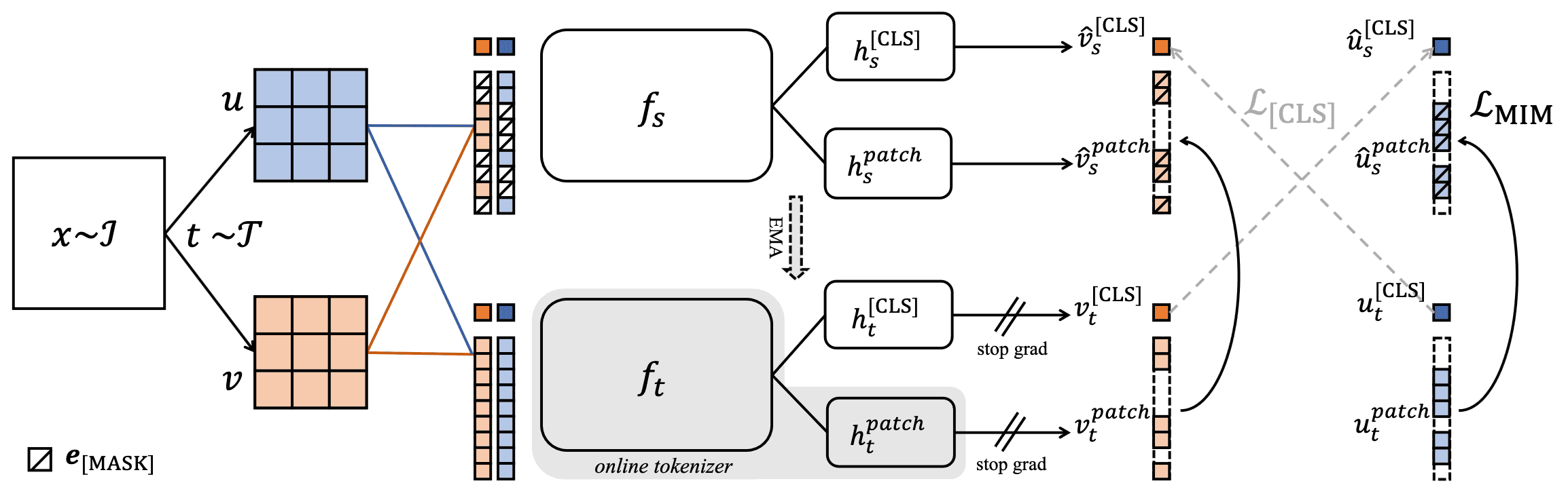
Given the training set $\mathcal{I}$, an image $\boldsymbol{x} \sim \mathcal{I}$ is sampled uniformly and two random augmentations are applied for invariance learning, yielding two distorted views $\boldsymbol{u}$ and $\boldsymbol{v}$. Then, these views are fed into teacher-student framework of $f_t$ and $f_s$, respectively attached $3$-layer MLP projection head $h_t$ and $h_s$, as follows:

1. Masked Image Modeling
   For normal patch tokens, block-wise masking of BEiT is applied on the two augmented views, yielding masked views $\hat{\boldsymbol{u}}$ and $\hat{\boldsymbol{v}}$. Denote by the masking indicator $m_i$; that is, the masked version $\hat{\boldsymbol{z}}$ of token sequence of an image $\boldsymbol{x} = \{ \boldsymbol{x}_i \}_{i=1}^N$ can be written as: $$ \hat{\boldsymbol{x}} = \{ \hat{\boldsymbol{x}}_i = (1 − m_i) \boldsymbol{x}_i + m_i \boldsymbol{e}^\texttt{[MASK]} \}_{i=1}^N $$ Then the target network $h_s^{\texttt{patch}} \circ f_s$ outputs the distribution $\hat{\boldsymbol{u}}_s^\texttt{patch} = \mathbb{P}_{\boldsymbol{\theta}_s}^{\texttt{patch}} (\hat{\boldsymbol{u}})$ for the masked view $\hat{\boldsymbol{u}}$, while the online tokenizer $h_t^{\texttt{patch}} \circ f_t$ outputs $\boldsymbol{u}_t^\texttt{patch} = \mathbb{P}_{\boldsymbol{\theta}_t}^{\texttt{patch}} (\boldsymbol{u})$ for the non-masked view $\boldsymbol{u}$.
   
   The training objective of MIM in iBOT is defined as the self-distillation loss that resembles DINO but is patch-level: $$ \mathcal{L}_{\texttt{MIM}} = - \frac{1}{2} \left( \sum_{i=1}^N m_i \cdot \mathbb{P}_{\boldsymbol{\theta}_t}^{\texttt{patch}} (\boldsymbol{u}_i) \cdot \log \mathbb{P}_{\boldsymbol{\theta}_s}^{\texttt{patch}} (\hat{\boldsymbol{u}}_i) + \sum_{j=1}^N m_j \cdot \mathbb{P}_{\boldsymbol{\theta}_t}^{\texttt{patch}} (\boldsymbol{v}_j) \cdot \log \mathbb{P}_{\boldsymbol{\theta}_s}^{\texttt{patch}} (\hat{\boldsymbol{v}}_j) \right) $$
   
2. Self-distillation for $\texttt{[CLS]}$
   To ensure that the online tokenizer is semantically meaningful, self-distillation is performed on the $\texttt{[CLS]}$ token of cross-view images. This allows visual semantics to be obtained through bootstrapping, as accomplished by the majority of self-supervised methods. Projection heads $h_t^{\texttt{[CLS]}}$ and is attached to the backbone $f_t$ and $f_s$, respectively, producing $\boldsymbol{v}^\texttt{[CLS]} = \mathbb{P}_{\boldsymbol{\theta}}^\texttt{[CLS]} (\boldsymbol{v})$. $$ \mathcal{L}_{\texttt{[CLS]}} = - \frac{1}{2} \left( \boldsymbol{v}_t^{\texttt{[CLS]}} \cdot \log \hat{\boldsymbol{u}}_s^{\texttt{[CLS]}} + \boldsymbol{u}_t^{\texttt{[CLS]}} \cdot \log \hat{\boldsymbol{v}}_s^{\texttt{[CLS]}} \right) $$

To further borrow the capability of semantics abstraction acquired from self-distillation on $\texttt{[CLS]}$ token, the parameters of projection heads for $\texttt{[CLS]}$ token and patch tokens are shared, i.e., $h_s^{\texttt{[CLS]}} = h_s^\texttt{patch}$ and $h_t^{\texttt{[CLS]}} = h_t^\texttt{patch}$ (They empirically demonstrated that it produces better results than using separate heads). Ultimately, these two losses are combined into a single loss:

\[\mathcal{L}_{\texttt{IBOT}} = \mathcal{L}_{\texttt{[CLS]}} + \mathcal{L}_{\texttt{MIM}}\]

where the objective is to reconstruct the masked tokens with the online tokenizers’ outputs as supervision.

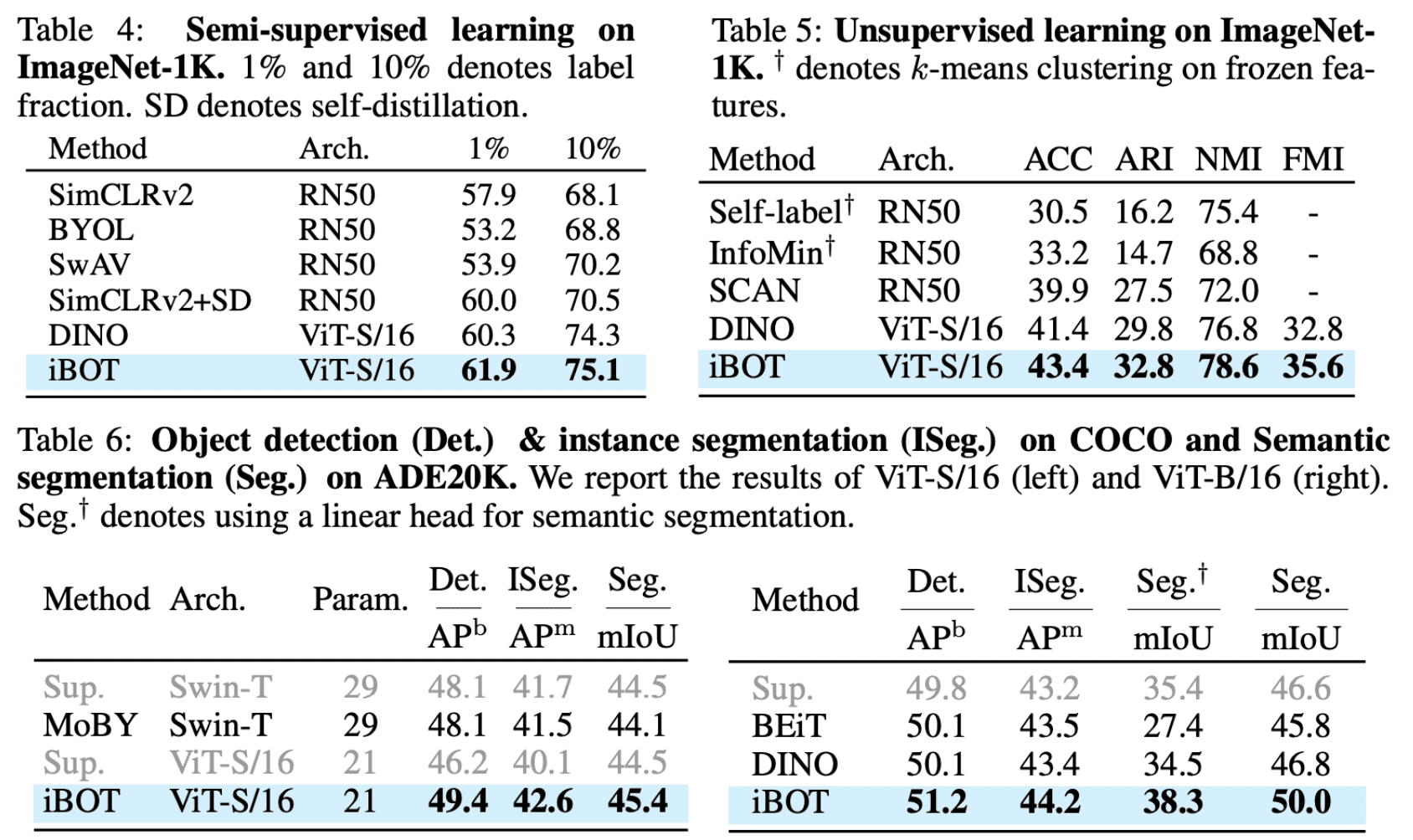
As a result, IBOT shows strong performance on linear probing as well as fine-tuning:

$\mathbf{Fig\ 18.}$ Linear Probing and Fine-tuning comparisons (Zhou et al., 2022)

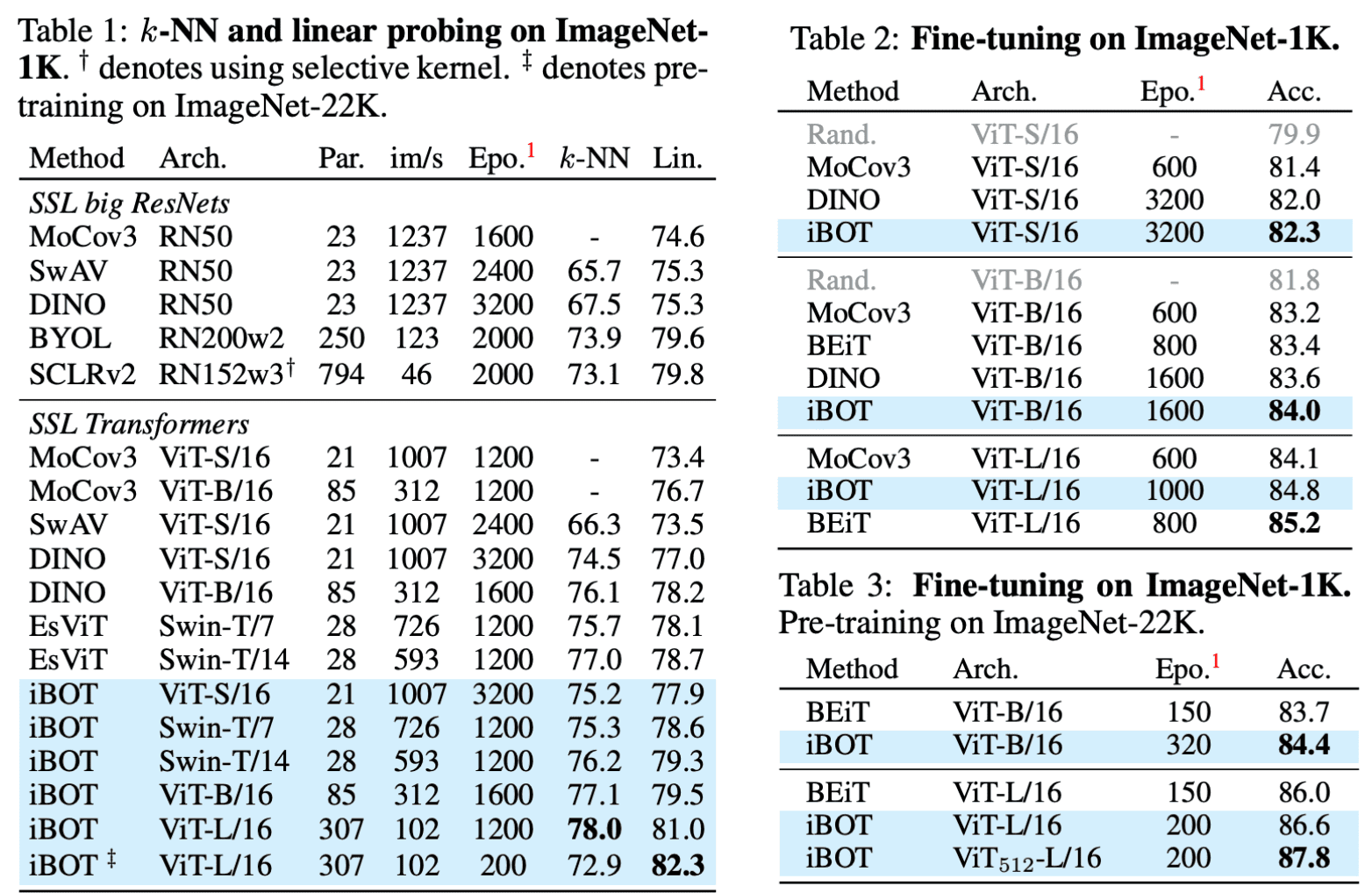
Moreover, IBOT demonstrates high transferability across various downstream tasks, including semi-supervised learning, unsupervised learning, object detection, and segmentation:

$\mathbf{Fig\ 19.}$ Transferability comparisons (Zhou et al., 2022)

Data2vec: Multi-modal Framework for Self-supervised Learning by MIM

While the general idea of self-supervised learning is consistent across modalities, the specific algorithms and objectives vary widely and are often not adaptable to other modalities, as they were developed with a single modality in mind. Data2vec, introduced by Baevski et al., 2022, is a framework for general self-supervised learning for images, speech, and text where the learning objective is identical across each modality.

$\mathbf{Fig\ 20.}$ Overview of data2vec (Baevski et al., 2022)

Data2vec combines masked prediction with the learning of latent target representations, generalizing the latter by using multiple network layers as targets. This approach demonstrates effectiveness across several modalities.

1. Modality-unified algorithm
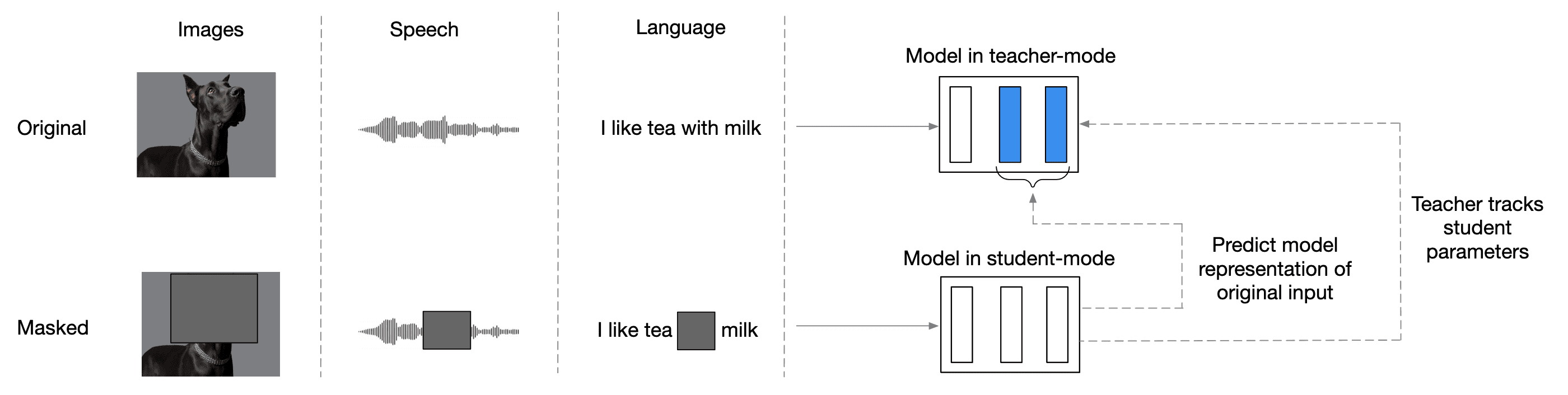
   The data2vec framework consists of two Transformer networks with teacher and student mode:
   
   • (1) Build representations of the full input data with the teacher model:
     • Theses representations will serve as targets in the learning task;
     • The teacher is an exponentially decaying average of the student; $$ \boldsymbol{\theta}_{\texttt{teacher}} \leftarrow \tau \boldsymbol{\theta}_{\texttt{teacher}} + (1-\tau) \boldsymbol{\theta}_{\texttt{student}} $$
   • (2) Encode the masked version of the input sample with the student model and predict the representations of original input from the teacher;
   Using the standard Transformer architecture for networks, the objective of data2vec is to predict the representations for time-steps masked in the student model. Specifically, the training targets $y_t$ are contextualized representations defined by the output of the top $K$ blocks of the teach network for time-steps masked in student-model: $$ y_t = \frac{1}{K} \sum_{l = L - K + 1}^L \hat{a}_t^l $$ where $\hat{a}_t^l$ denotes the normalized output of block $l$ at time-step $t$. Normalizing the targets helps prevent the model from collapsing into a constant representation for all time-steps, and it also prevents layers with high norms from dominating the target features. And the target objective is smooth-$\ell_1$ loss between $y$ and the prediction $f(x)$ of student model at $t$: $$ \mathcal{L} (y_t, f_t(x))= \begin{cases} \frac{1}{2}\left(y_t-f_t(x)\right)^2 / \beta & \left|y_t-f_t(x)\right| \leq \beta \\ \left(\left|y_t-f_t(x)\right|-\frac{1}{2} \beta\right) & \text { otherwise } \end{cases} $$

   

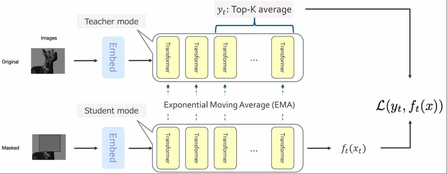
   $\mathbf{Fig\ 21.}$ Modality-unified algorithm of data2vec
   
   
2. Modality-specified data processing and masking strategy
   Since different modalities have vastly different inputs, data2vec employs modality-specific data processing and masking strategies.
   • Image processing
     • (Input embed) Embed images of $224 \times 224$ pixels as patches of $16 \times 16$ pixels
     • (Masking) BEiT (block-wise) masking strategy with $60\%$ masking ratio
   • Speech processing
     • (Input embed) Sample with $16\textrm{kHz}$ then forward seven temporal convolutions
     • (Masking) Mask $49\%$ of all time-steps
   • Image processing
     • (Input embed) The input data is tokenized using a byte-pair encoding (BPE)
     • (Masking) BERT masking strategy to $15\%$ of uniformly selected tokens:
       • $80\%$ are replaced by a learned mask token $\texttt{[M]}$;
       • $10\%$ are left unchanged;
       • $10\%$ are replaced by randomly selected vocabulary token;

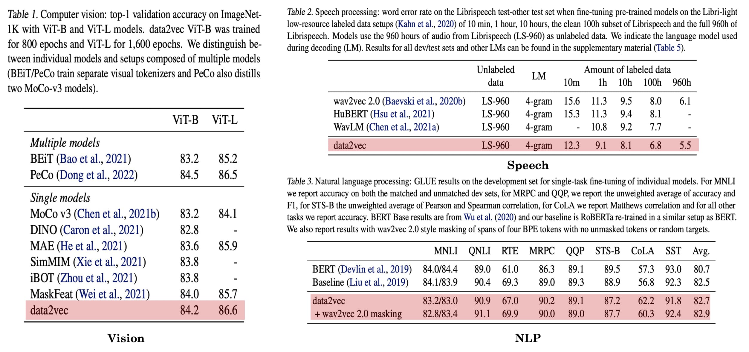
As a result, data2vec shows a new state-of-the-art or competitive performance to predominant approaches on three domains:

• Vision task: ImageNet classification
• Speech task: Word error rate (smaller is better) on the Librispeech dataset
• NLP task: GLEU benchmark

$\mathbf{Fig\ 22.}$ Comparisons of data2vec in different modalities (Baevski et al., 2022)

References

[1] Bao et al., “BEIT: BERT Pre-Training of Image Transformers”, ICLR 2022
[2] He et al., “Masked Autoencoders Are Scalable Vision Learners”, CVPR 2022
[3] Xie et al., “SimMIM: A Simple Framework for Masked Image Modeling”, CVPR 2022
[4] Zhou et al., “IBOT: Image BERT Pre-Training with Online Tokenizer”, ICLR 2022
[5] Baevski et al., “data2vec: A General Framework for Self-supervised Learning in Speech, Vision and Language”, ICML 2022 Oral
[6] Zhang et al., “A Survey on Masked Autoencoder for Self-supervised Learning in Vision and Beyond” IJCAI 2023