[Representation Learning] Explainability of CLIP

Most existing visualization methodologies for vision models, such as ZFNet and CAM, are designed for full-supervised models with single modality. When I attempted to visualize the attention activation of CLIP using attention rollout, self-attention quality of CLIP was very bad and difficult to interpret, leading to confused results that focus on partial regions.

$\mathbf{Fig\ 1.}$ Visualizing CLIP with Attention Rollout

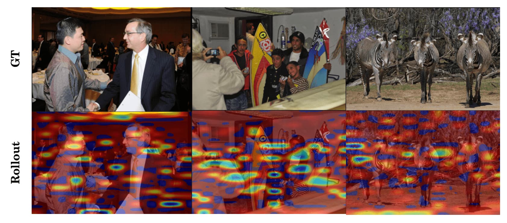
Motivated by my experiments, in this post, I have summarized some efforts that aim to improve the explainability of CLIP.

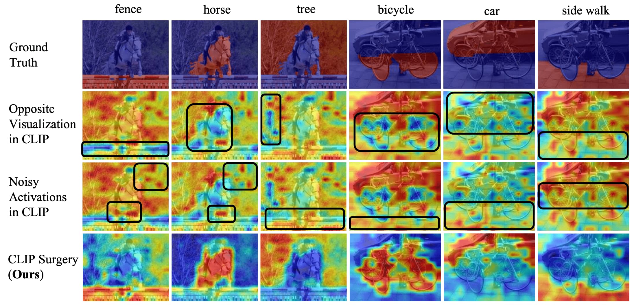
Problem: Opposite Visualization & Noisy Activation

When we visualize the class activation maps of CLIP, two main issues are observed:

1. Opposite Visualization
   visualization results that are opposite to the ground-truth
2. Noisy Activations
   the obvious highlights on background regions, which often appear on irrelevant regions in spot shape

$\mathbf{Fig\ 2.}$ Opposite Visualization and Noisy Activations (Li et al. 2023)

ECLIP & RCLIP

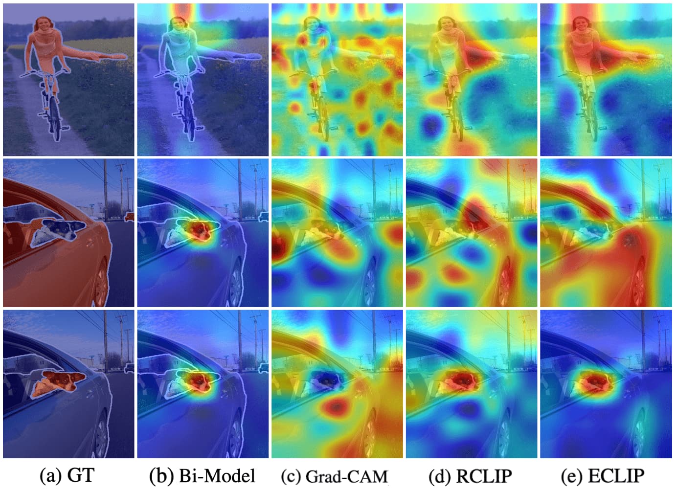
The opposite visualization of CLIP was first reported by Li et al. 2022. It demonstrated that the devil is in the pooling part of visual encoder: average pooling and attention pooling trigger feature shift that forces background features to be shifted to foreground regions and vice versa, thereby resulting erroneous visualization.

$\mathbf{Fig\ 3.}$ Left: Visualization results shown that max pooling solve the problem. Right: Illustration of feature shift and semantic shift (d) on CLIP ViT-B/16. Blue points indicate features shifted from background to foreground, and opposite for red points. (Li et al. 2022)

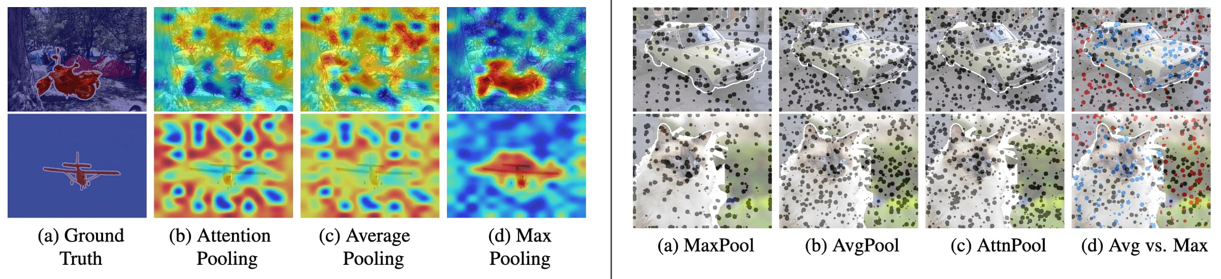
They argued to use max pooling instead of average pooling, proposing the new arcitecture called Explainable CLIP (ECLIP). It transforms the features from CLIP encoders with max pooling and linear projection, where linear projections $\phi_i$ and $\phi_t$ are fine-tuned with freezing the CLIP encoders.

$\mathbf{Fig\ 4.}$ Architecture of ECLIP (Li et al. 2022)

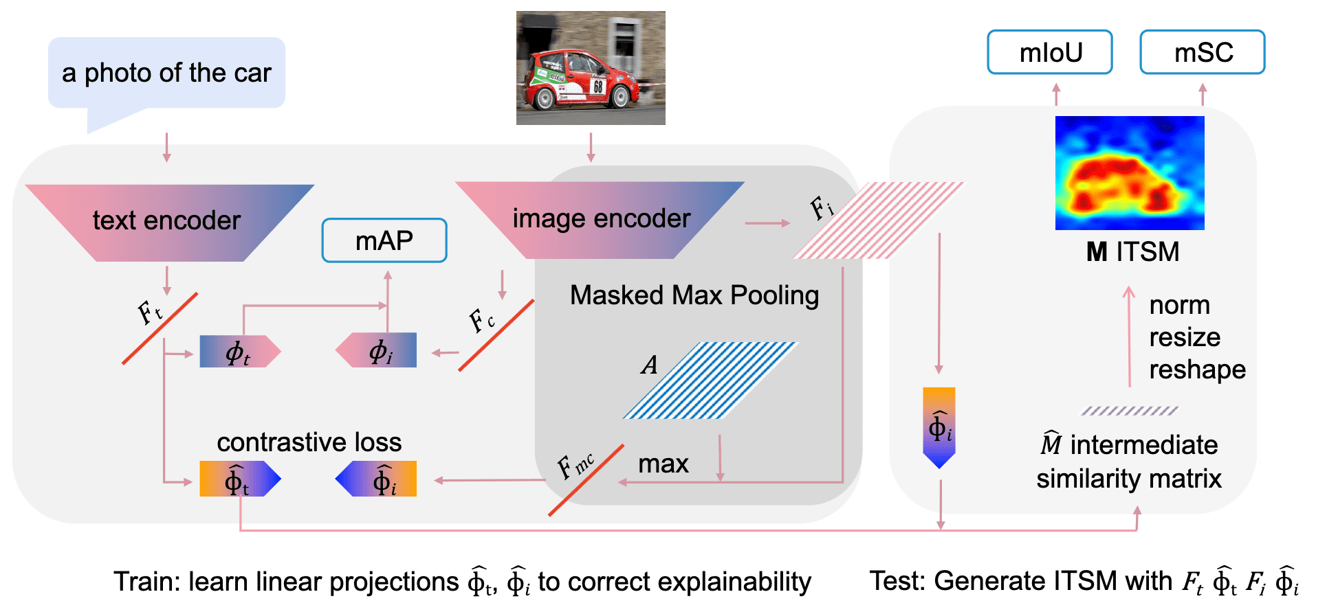
Also, they claimed that the opposite visualization can be alleviated without max pooling by simply reversing image-text similarity map (ITSM) $\mathbf{M} \in \mathbb{R}^{H \times W \times N}$:

\[\mathbf{M} \to \mathrm{abs}(\mathbf{I} - \mathbf{M})\]

where $\phi_i$ and $\phi_t$ are linear projections trained from ECLIP and

\[\begin{aligned} \hat{M} & = \left( \frac{f^{\texttt{img_enc}} (\mathbf{x}_i) \cdot \phi_i}{\Vert f^{\texttt{img_enc}} (\mathbf{x}_i) \cdot \phi_i \Vert_2} \right) \cdot \left( \frac{f^{\texttt{txt_enc}} (\mathbf{x}_t) \cdot \phi_t}{\Vert f^{\texttt{txt_enc}} (\mathbf{x}_t) \cdot \phi_t \Vert_2} \right)^\top \\ \mathbf{M} & = \texttt{norm}(\texttt{resize}(\texttt{reshape} (\hat{M}))) \end{aligned}\]

And such approach is named Reversed CLIP (RCLIP).

$\mathbf{Fig\ 5.}$ Visualization comparison between conventional methods (Li et al. 2022)

CLIP Surgery

Li et al. 2023 hypothesized that these issues stem from the following reasons and proposed a simple inference modification without any training or fine-tuning, termed CLIP Surgery:

1. Opposite Visualization
   the parameters (query $\mathbf{q}$ and key $\mathbf{k}$) in the self-attention module heavily focus on opposite semantic regions;
   $\Rightarrow$ Architecture Surgery: estabilish dual paths with V-V Self-Attention
2. Noisy Activations
   redundant features in CLIP interrupts the visualization;
   $\Rightarrow$ Feature Surgery: define redundant features with the mean features along the class dimension and remove them

Architecture Surgery

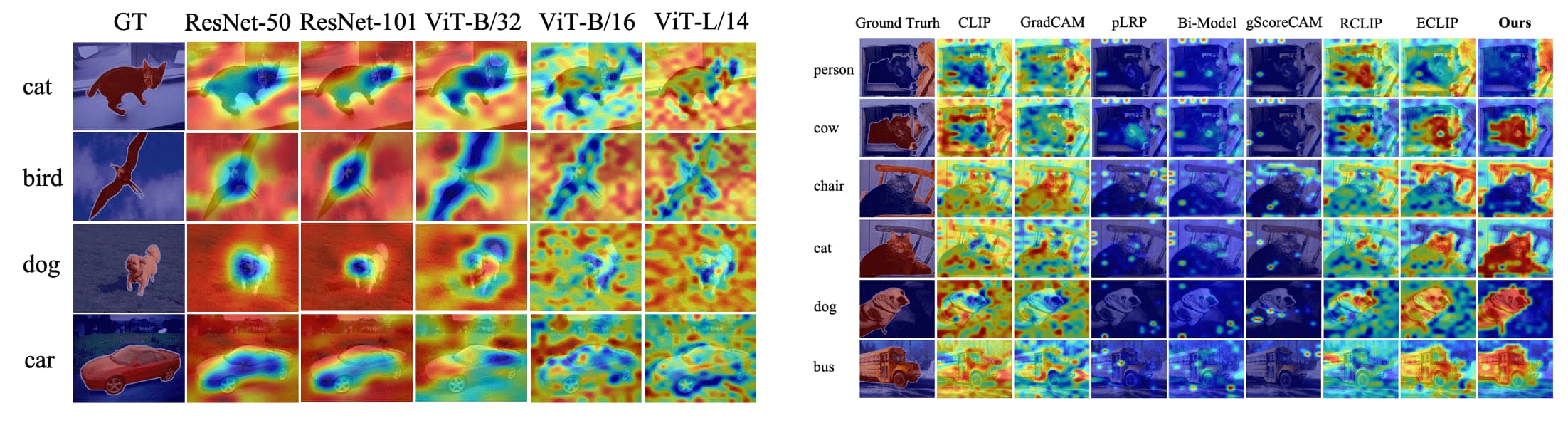
The authors generated similarity maps $\mathbf{M}$ of CLIP, and observe that the most prominent problem is the opposite visualization. In particular, when identifying a target category, CLIP tends to prioritize background regions over foreground regions, which contradicts human perception. This is also observed across various backbones (ResNets and ViTs), and occurs in multiple existing visualization methods, too.

\[\mathbf{M} = \texttt{norm}\left(\texttt{resize}\left(\texttt{reshape} \left( \frac{f^\texttt{img_enc} (\mathbf{x}_i)}{\Vert f^\texttt{img_enc} (\mathbf{x}_i) \Vert_2} \left(\frac{f^\texttt{txt_enc} (\mathbf{x}_t)}{\Vert f^\texttt{txt_enc} (\mathbf{x}_t) \Vert_2}\right)^\top \right)\right)\right) \in \mathbb{R}^{H \times W \times N_t}\]

where $\texttt{reshape}$ and $\texttt{resize}$ operator convert the number of image tokens $N_i$ to the image size $H \times W$.

$\mathbf{Fig\ 6.}$ Visualization comparison between conventional methods (Li et al. 2023)

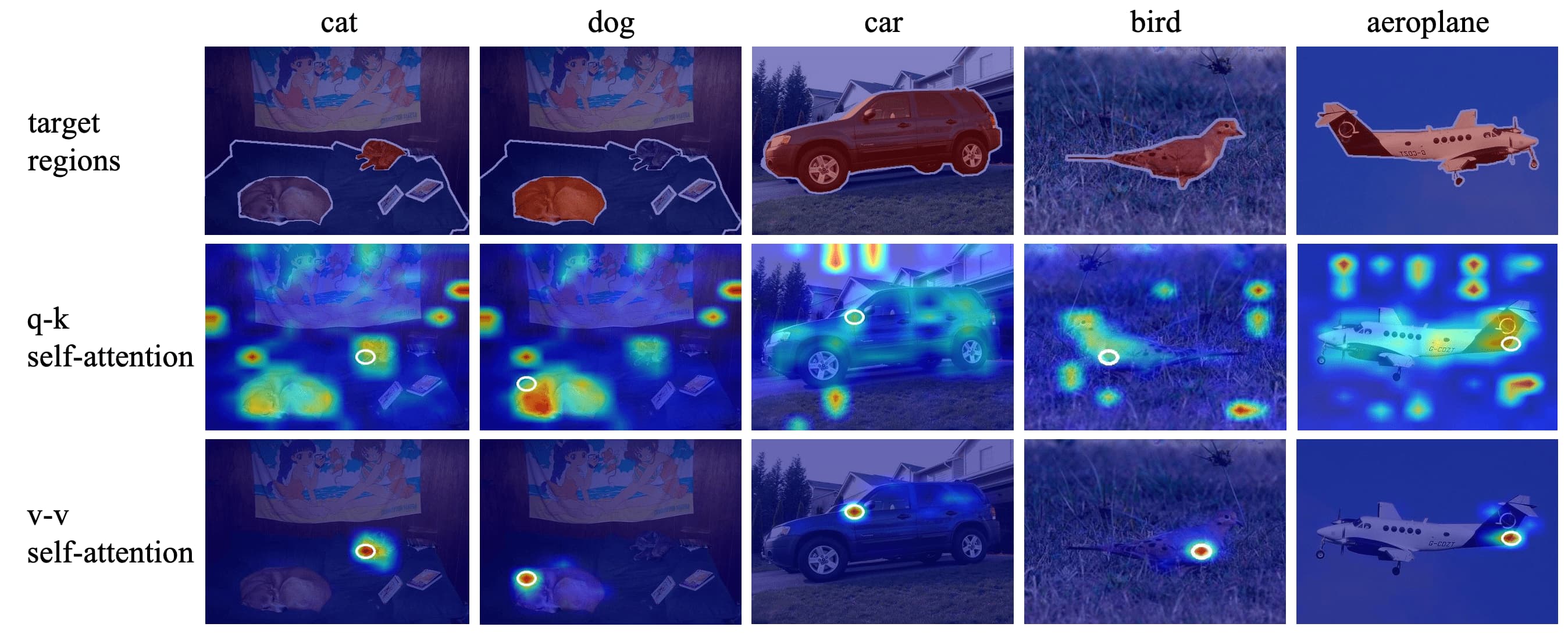
They claimed that the parameters key and query in self-attention link features from opposite semantic regions. Specifically, the original query-key self-attention of CLIP computes its attention score as:

\[\texttt{Attn}_{\mathbf{qk}} = \texttt{softmax}(\frac{1}{c} \mathbf{Q} \mathbf{K}^\top) \cdot \mathbf{V}\]

Instead, they proposed value-value self-attention which computes the attention score as follows:

\[\texttt{Attn}_{\mathbf{vv}} = \texttt{softmax}(\frac{1}{c} \mathbf{V} \mathbf{V}^\top) \cdot \mathbf{V}\]

In qualitative comparison, the original q-k attention focuses extensively on semantically opposite regions. This results in a confused attentiom map, where background information is embedded into features of foreground tokens. Conversely, the proposed v-v attention is effective; it ensures that the cosine distance on itself is the highest and highlights nearby tokens, rather than paying attention to irrelevant regions. This evidence suggests that problematic parameters in self-attention lead to confused relationships, causing tokens to be identified with opposite meanings.

$\mathbf{Fig\ 7.}$ Visual comparison between q-k self-attention of CLIP and v-v self-attention (Li et al. 2023)

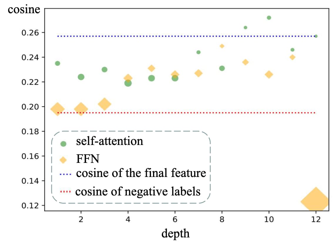
Additionally, the explainability of CLIP for multiple modules are also investigated in the paper via cosine of angle bettwen text feature $\mathbf{F}_t$ and feature of a certain module at the class token $\hat{\mathbf{F}}_c$:

\[\frac{\mathbf{F}_t \cdot \hat{\mathbf{F}}_c}{\Vert \mathbf{F}_t \Vert_2 \cdot \Vert \hat{\mathbf{F}}_c \Vert_2}\]

FFN modules exhibit larger gaps than self-attention modules when computing the cosine of the angle with the final classification feature. Notably, the last FFN returns a feature with a cosine of $0.1231$, which is much farther than the cosine of negative labels. Moreover, features from the first three FFNs are very close to those of negative labels. This suggests that FFNs push features towards negatives when identifying positives, thereby impairing the model performance.

$\mathbf{Fig\ 8.}$ Cosine of angles for self-attentions and FFNs at different depths (Li et al. 2023)

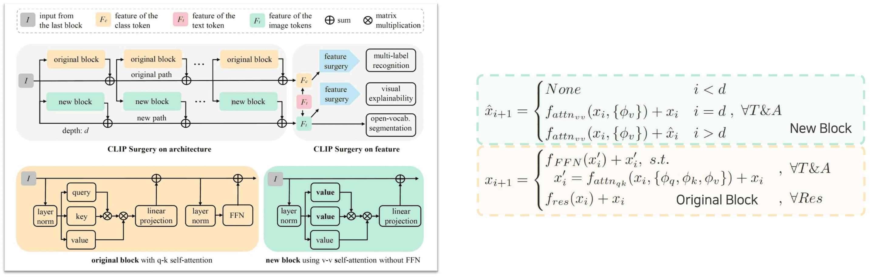
With the analysis above, the authors defined the Architecture Surgery with dual paths to merge features from multiple v-v self-attention layers while maintaining stable input and retaining original features for the classification task without FFNs.

In particular, for the hyperparameter depth $d$, the original visual encoder blocks remain unchanged, incorporating q-k self-attention $f_{\texttt{qk-attn}}$ and FFNs $f_{\texttt{FFN}}$. Beyond the depth $d$, the feature from original block of the CLIP path is summed feature-wise with the output of new block, which consists of the v-v self-attention $f_{\texttt{vv-attn}}$ and a linear projection layer without FFNs. This dual path allows merging features from multiple layers without back-propagation, thereby being faster and efficient.

$\mathbf{Fig\ 9.}$ CLIP Architecture Sugery: V-V Self-Attention + w/o FFN (Li et al. 2023)

Feature Surgery

Noisy activations appear as highlights in spot shapes uniformly at unexpected positions instead of discriminative areas. It is universal for varied backbones and methods, including Grad-CAM for CNNs and Bi-Modal for multi-modal ViTs.

$\mathbf{Fig\ 10.}$ Noisy Activations (Li et al. 2023)

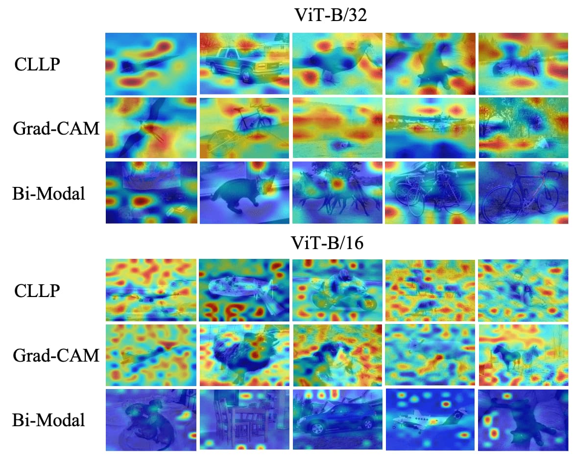
Interestingly, noisy activations are uniform across labels and even occur with an empty prompt. This indicates that false predictions and related contexts, such as “lake” and “boat”, cannot account for the cause of these noisy activations.

$\mathbf{Fig\ 11.}$ Noisy activations are similar across labels and occur in the empty prompt. (Li et al. 2023)

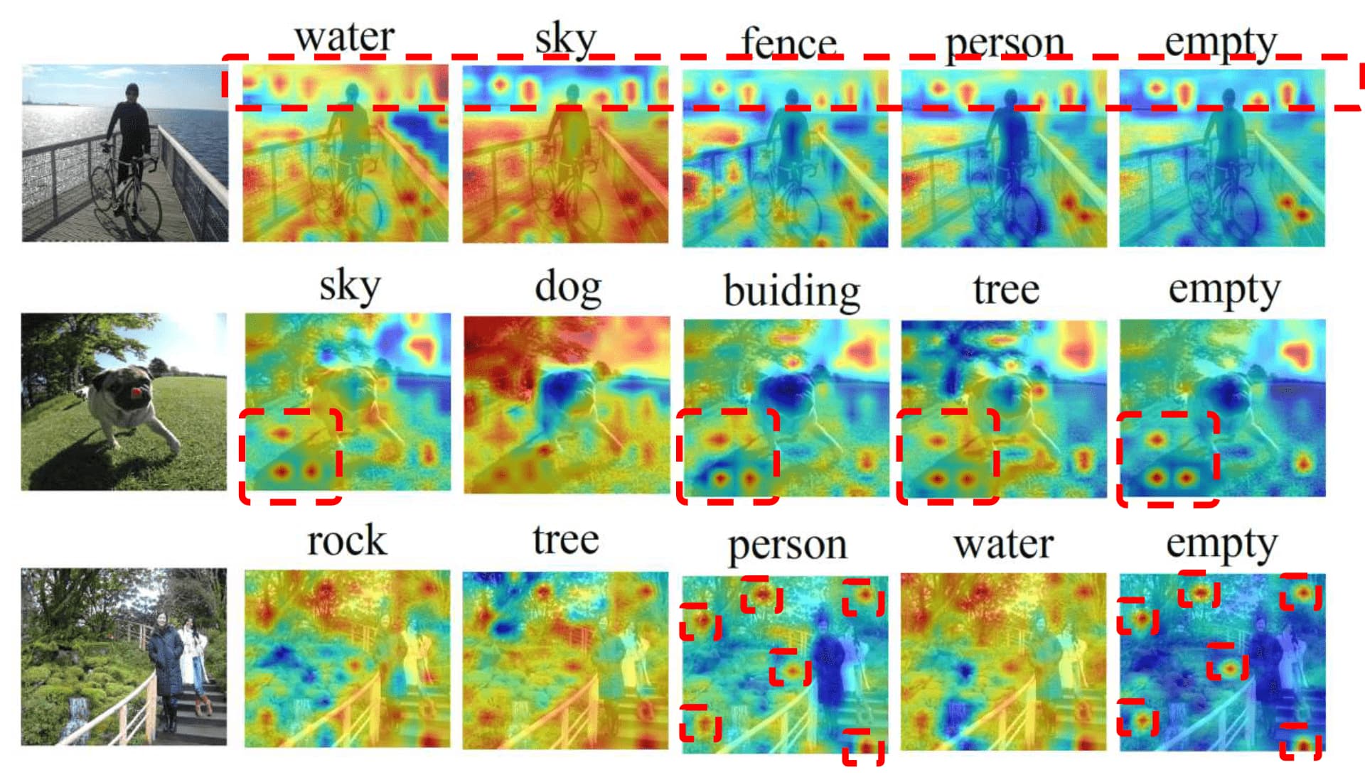
The authors claimed that noisy activations are caused by redundant features in CLIP. Specifically, CLIP learns to recognize numerous categories through natural language, which means that only a few features are activated for a particular class, while other features remain inactive for the rest of other classes. Consequently, these non-activated features become redundant and occupy a significant portion of the feature space. And the noisy activations observed in the similarity maps are a direct result of these redundant features being activated.

Feature Surgery aims to remove such redundant features by defining redundant feature using the mean features along the class dimension. For given image features $\mathbf{F}_i \in \mathbb{R}^{N_i \times C}$ and text features $\mathbf{F}_t \in \mathbb{R}^{N_t \times C}$, it firstly multiplied features $\mathbf{F}_m \in \mathbb{R}^{N_i \times N_t \times C}$ by $\texttt{expand}$ operation and element-wise multiplication:

\[\mathbf{F}_m = \frac{\texttt{expand}(\mathbf{F}_i, N_i \times N_t \times C)}{\Vert \texttt{expand}(\mathbf{F}_i, N_i \times N_t \times C) \Vert_2} \odot \frac{\texttt{expand}(\mathbf{F}_t, N_i \times N_t \times C)}{\Vert \texttt{expand}(\mathbf{F}_t, N_i \times N_t \times C) \Vert_2}\]

To emphasize activated portions of the feature, it calculates category weight $\mathbf{w} \in \mathbb{R}^{1 \times N_t}$ by average normalizing similarity score $\mathbf{s} \in \mathbb{R}^{1 \times N_t}$ between class token feature $\mathbf{F}_c \in \mathbb{R}^{1 \times C}$ and text features:

\[\mathbf{w} = \frac{\mathbf{s}}{\texttt{avg}(\mathbf{s})} \quad \text{ where } \quad \mathbf{s} = \texttt{softmax} \left( \tau \cdot \frac{\mathbf{F}_c}{\Vert \mathbf{F}_c \Vert_2} \left(\frac{\mathbf{F}_t}{\Vert \mathbf{F}_t \Vert_2}\right)^\top \right)\]

where $\tau$ is the logit scale for $\texttt{softmax}$. Then it defines the redundant features \(\mathbf{F}_r \in \mathbb{R}_{N_i \times 1 \times C}\) as follows:

\[\mathbf{F}_r = \texttt{mean} (\mathbf{F}_m \odot \texttt{expand}(\mathbf{w}))\]

Defined redundant feature is expanded to the same shape as multiplied features $\mathbf{F}_m$ to compute cosine similarity $\mathbf{S} \in \mathbb{R}^{N_i \times N_t}$, which is utilized to compute the similarity map $\mathbf{M} \in \mathbb{R}^{H \times W \times N_t}$:

\[\mathbf{M} = \texttt{norm}(\texttt{resize}(\texttt{reshape} (\mathbf{S}))) \; \text{ where } \; \mathbf{S} = \texttt{sum}(\mathbf{𝑭}_m - \texttt{expand}(\mathbf{F}_r) )\]

References

[1] Li et al. “Exploring Visual Explanations for Contrastive Language-Image Pre-training”, arXiv preprint 2022
[2] Li et al. “CLIP Surgery for Better Explainability with Enhancement in Open-Vocabulary Tasks” arXiv preprint 2023