[Generative Model] Preference Optimization for Diffusion Models
Training generative models to understand and predict human preferences is highly complex task. LLMs, for example, can be “prompted” to perform a range of NLP tasks by providing examples as input. Traditional methods like supervised fine-tuning often require assigning supervision labels to data, which imposes significant burden to human. Futhermore, the training objectives of many recent models are misaligned with human goals, as they differ from the objective of “following the user instructions helpfully and safely”. Therefore, these models frequently exhibit unintended behaviors such as hallucination, toxic AI, or simply not following user instructions.
Preference optimization has drawn wide attention as an alternative approach that simplifies this process and aligns more with human preferences. By focusing on comparing and ranking candidate human responses, it enables models to better capture the nuances of human judgment.
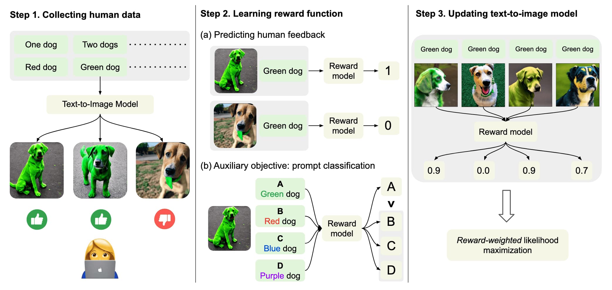
Preliminaries: Preference Optimization of Language Model
Human preference learning of generative models has been extensively studied in LLMs first. To understand preference optimization of diffusion models, it is essential to familiarize oneself with the foundational research in LLMs.
RLHF (Reinforcement Learning from Human Feedback)
Reinforcement Learning from Human Feedback (RLHF), first proposed by Cristiano et al. 2017, stems from the field of RL but recently serves as a fine-tuning technique to enhance AI models’ performance based on human feedback. This is well-exemplified by Ouyang et al. 2023, which proposed InstructGPT, a GPT fine-tuned via RLHF.
The key components of InstructGPT include the language model being fine-tuned, the reward model that assesses the language model’s outputs, and the human feedback that guides the reward model. Viewing the language model as the policy, it is trained using RL algorithms such as PPO. This process ensures that the language model generates outputs that are more aligned with human preferences.

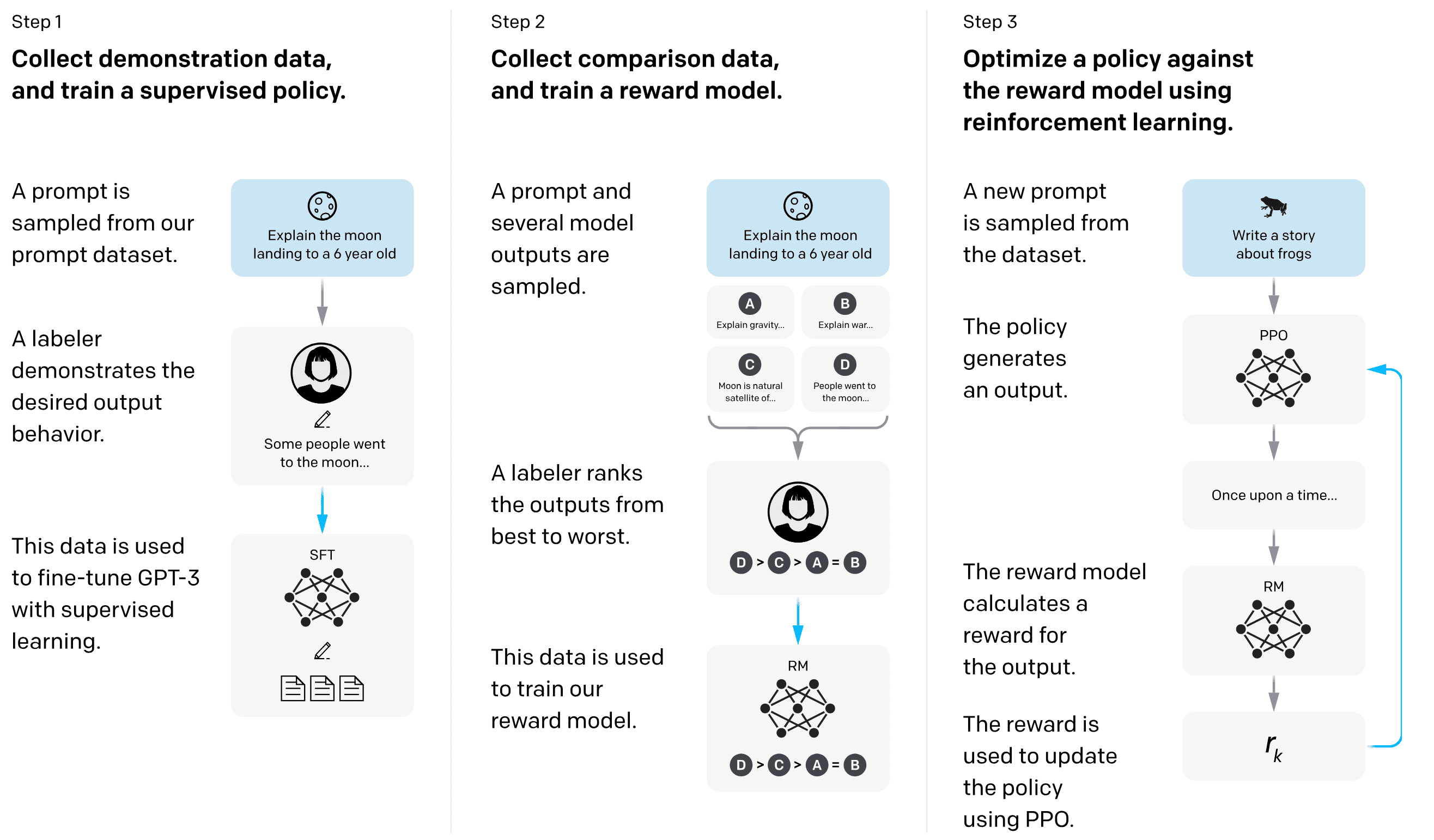
The InstructGPT consists of three main training stages:
- Supervised Fine-tuning (SFT)
The authors collected a dataset $\mathcal{D}_\texttt{demonstration} = \{ (\mathbf{x}, \mathbf{y})^i \}_{i=1}^M$ of human-written demonstrations of the desired output behavior on input prompts. For example: $$ \begin{aligned} & \texttt{Input: } \textrm{Explain the moon landing to a 6 year old.} \\ & \texttt{Output: } \textrm{A long time ago, some brave astronauts decided to go on a big adventure to the Moon... (written by human)} \end{aligned} $$ The InstructGPT is first trained by supervised learning with this demonstration dataset. We will denote this supervised fine-tuned model as $\pi_\texttt{SFT}$. - Reward Modeling (RM)
To model the reward function $r_\boldsymbol{\phi}$, the authors also collected the human preference dataset $\mathcal{D} = \{ (\mathbf{x}, \mathbf{y}_w, \mathbf{y}_l)^i \}_{i=1}^N$. That is, for input prompt $\mathbf{x}$, $\mathbf{y}_w$ is the completion preferred by human labelers out of the pair $(\mathbf{y}_w, \mathbf{y}_l)$. Then, $r_\boldsymbol{\phi}$ is trained using the following cross-entropy loss: $$ \mathcal{L}_\texttt{reward} (\boldsymbol{\phi}) \propto - \mathbb{E}_{(\mathbf{x}, \mathbf{y}_w, \mathbf{y}_l) \sim \mathcal{D}} \left[ \log \sigma \left( r_\boldsymbol{\phi} (\mathbf{x}, \mathbf{y}_w) - r_\boldsymbol{\phi} (\mathbf{x}, \mathbf{y}_l) \right) \right] $$ where $\sigma$ is the sigmoid function. Note that it computes the probabilities that the reward model assigns a higher reward to $\mathbf{y}_w$ than to $\mathbf{y}_l$ using Bradley-Terry model: $$ p (\mathbf{y}_w \succ \mathbf{y}_l \vert \mathbf{x}) = \sigma \left( r_\boldsymbol{\phi} (\mathbf{x}, \mathbf{y}_w) - r_\boldsymbol{\phi} (\mathbf{x}, \mathbf{y}_l) \right) = \frac{\exp \left( r_\boldsymbol{\phi} (\mathbf{x}, \mathbf{y}_w) \right)}{\exp \left( r_\boldsymbol{\phi} (\mathbf{x}, \mathbf{y}_w) \right) + \exp \left( r_\boldsymbol{\phi} (\mathbf{x}, \mathbf{y}_l) \right)} $$ And $\mathcal{L}_\texttt{reward}$ is maximizing this probability. Finally, since the loss is shift-invariant in reward, the reward model is normalized using a bias so that the labeler demonstrations achieve a mean score of $0$. - Fine-tuning with Reinforcement Learning (RL)
Finally, considering the InstructGPT as a policy $\pi_\boldsymbol{\theta}$ and freezed $\pi_\texttt{SFT}$ as an old policy $\pi_{\boldsymbol{\theta}_\texttt{old}}$, the language model is further fine-tuned using PPO algorithm in the bandit environment equipped with our reward $r_\boldsymbol{\phi}$. Recall that the PPO objective (Schulman et al. 2017) is given by: $$ \max_\boldsymbol{\theta} \; \mathbb{E}_t \left[ \frac{\pi_\boldsymbol{\theta} (\mathbf{a}_t \vert \mathbf{s}_t)}{\pi_{\boldsymbol{\theta}_\texttt{old}} (\mathbf{a}_t \vert \mathbf{s}_t)} \hat{A}^\boldsymbol{\theta_\texttt{old}} (\mathbf{s}_t, \mathbf{a}_t) - \beta \cdot \mathrm{KL} \left(\pi_{\boldsymbol{\theta}_\texttt{old}} (\cdot \vert \mathbf{s}_t) \Vert \pi_\boldsymbol{\theta} (\cdot \vert \mathbf{s}_t) \right) \right] $$ Then, the authors simplified this objective in our bandit case as follows (but not exactly equivalent to the PPO objective), without any state transition and timesteps: $$ \mathcal{L}_\texttt{RL} (\boldsymbol{\theta}) = \mathbb{E}_{(\mathbf{x}, \mathbf{y}) \sim \mathcal{D}_{\pi_\boldsymbol{\theta}}} \left[ r_\boldsymbol{\phi} (\mathbf{x}, \mathbf{y}) - \beta \cdot \log \left ( \frac{\pi_\boldsymbol{\theta} (\mathbf{y} \vert \mathbf{x})}{\pi_\texttt{SFT} (\mathbf{y} \vert \mathbf{x})} \right) \right] $$ Note that the advantage function $\hat{A}$ is simply replaced by $r_\boldsymbol{\phi}$ since we normalized before training as claimed above. Therefore, we can perform the optimization with its surrogate objective function such as CLIP or something else.
DPO (Direct Preference Optimization)
RLHF first fit reward model to a dataset of prompts and human preferences over pairs of responses, and then use RL to find a policy that maximizes the learned reward. And such RLHF pipeline is considerably more complex than supervised learning, involving training multiple LMs and sampling from the LM policy in the loop of training that incur significant computational costs. Furthermore, RLHF often exhibit unstable behavior and mode-collapse to single high-reward answers.
In contrast, Direct Preference Optimization (DPO) proposed by Rafailov et al. 2023 directly optimizes for the policy best satisfying the preferences with a simple classification objective, fitting an implicit reward model whose corresponding optimal policy can be extracted in closed form. Consequently, they showed that the language model can function as a reward model to understand human preference in an implicative way through DPO formulation.

Change-of-variables for implicit reward
DPO avoids filling an explicit reward model by using change-of-variables technique, which can be derived from the analytical mapping from reward functions to optimal policies:
\[\begin{aligned} & \max_{\boldsymbol{\theta}} \; \mathbb{E}_{(\mathbf{x}, \mathbf{y}) \sim \mathcal{D}_{\pi_\boldsymbol{\theta}}} \left[ r_\boldsymbol{\phi} (\mathbf{x}, \mathbf{y}) - \beta \cdot \log \left ( \frac{\pi_\boldsymbol{\theta} (\mathbf{y} \vert \mathbf{x})}{\pi_\texttt{SFT} (\mathbf{y} \vert \mathbf{x})} \right) \right] \\ = & \; \min_{\boldsymbol{\theta}} \; \mathbb{E}_{(\mathbf{x}, \mathbf{y}) \sim \mathcal{D}_{\pi_\boldsymbol{\theta}}} \left[ \log \left ( \frac{\pi_\boldsymbol{\theta} (\mathbf{y} \vert \mathbf{x})}{\pi_\texttt{SFT} (\mathbf{y} \vert \mathbf{x})} \right) - \frac{1}{\beta} r_\boldsymbol{\phi} (\mathbf{x}, \mathbf{y}) \right] \\ = & \; \min_{\boldsymbol{\theta}} \mathbb{E}_{(\mathbf{x}, \mathbf{y}) \sim \mathcal{D}_{\pi_\boldsymbol{\theta}}} \left[ \log \left ( \frac{\pi_\boldsymbol{\theta} (\mathbf{y} \vert \mathbf{x})}{\frac{1}{Z (\mathbf{x})} \pi_\texttt{SFT} (\mathbf{y} \vert \mathbf{x}) \exp \left( \frac{1}{\beta} r_\boldsymbol{\phi} (\mathbf{x}, \mathbf{y}) \right)} \right) - \log Z (\mathbf{x}) \right] \\ = & \; \min_{\boldsymbol{\theta}} \mathbb{E}_{\mathbf{x} \sim \mathcal{D}} \left[ \mathrm{KL} \left(\pi_\boldsymbol{\theta} (\cdot \vert \mathbf{x}) \middle\Vert \frac{1}{Z (\mathbf{x})} \pi_\texttt{SFT} (\cdot \vert \mathbf{x}) \exp \left( \frac{1}{\beta} r_\boldsymbol{\phi} (\mathbf{x}, \cdot) \right) \right) - \log Z (\mathbf{x}) \right] \\ & \therefore \pi^* (\mathbf{y} \vert \mathbf{x}) = \frac{1}{Z (\mathbf{x})} \pi_\texttt{SFT} (\mathbf{y} \vert \mathbf{x}) \exp \left( \frac{1}{\beta} r_\boldsymbol{\phi} (\mathbf{x}, \mathbf{y}) \right) \end{aligned}\]where $Z (\mathbf{x}) = \sum_\mathbf{y} \pi_\texttt{SFT} (\mathbf{y} \vert \mathbf{x}) \exp \left( \frac{1}{\beta} r_\boldsymbol{\phi} (\mathbf{x}, \mathbf{y}) \right)$ is the partition function. This gives us the following implicit formulation of reward model:
\[r (\mathbf{x}, \mathbf{y}) = \beta \cdot \log \frac{\pi_\boldsymbol{\theta} (\mathbf{y} \vert \mathbf{x})}{\pi_\texttt{SFT} (\mathbf{y} \vert \mathbf{x})} + \beta \cdot \log Z (\mathbf{x})\]Thus, the optimal RLHF policy $\pi^*$ under the Bradley-Terry model satisfies the preference model:
\[\begin{gathered} p (\mathbf{y}_w \succ \mathbf{y}_l \vert \mathbf{x}) = \sigma \left( r_\boldsymbol{\phi} (\mathbf{x}, \mathbf{y}_w) - r_\boldsymbol{\phi} (\mathbf{x}, \mathbf{y}_l) \right) = \frac{\exp \left( r_\boldsymbol{\phi} (\mathbf{x}, \mathbf{y}_w) \right)}{\exp \left( r_\boldsymbol{\phi} (\mathbf{x}, \mathbf{y}_w) \right) + \exp \left( r_\boldsymbol{\phi} (\mathbf{x}, \mathbf{y}_l) \right)} \\ \Big\Downarrow \\ p (\mathbf{y}_w \succ \mathbf{y}_l \vert \mathbf{x}) = \frac{1}{1 + \exp \left( \beta \cdot \log \dfrac{\pi^* (\mathbf{y}_l \vert \mathbf{x})}{\pi_\texttt{SFT} (\mathbf{y}_l \vert \mathbf{x})} - \beta \cdot \log \dfrac{\pi^* (\mathbf{y}_w \vert \mathbf{x})}{\pi_\texttt{SFT} (\mathbf{y}_w \vert \mathbf{x})} \right)} \end{gathered}\]Consequently, our policy objective becomes:
\[\begin{gathered} \mathcal{L}_\texttt{reward} (\boldsymbol{\phi}) = - \mathbb{E}_{(\mathbf{x}, \mathbf{y}_w, \mathbf{y}_l) \sim \mathcal{D}} \left[ \log \sigma \left( r_\boldsymbol{\phi} (\mathbf{x}, \mathbf{y}_w) - r_\boldsymbol{\phi} (\mathbf{x}, \mathbf{y}_l) \right) \right] \\ \Big\Downarrow \\ \mathcal{L}_\texttt{DPO} (\boldsymbol{\theta}) = - \mathbb{E}_{(\mathbf{x}, \mathbf{y}_w, \mathbf{y}_l) \sim \mathcal{D}} \left[ \log \sigma \left( \beta \cdot \log \frac{\pi_\boldsymbol{\theta} (\mathbf{y}_w \vert \mathbf{x})}{\pi_\texttt{SFT} (\mathbf{y}_w \vert \mathbf{x})} - \beta \cdot \log \frac{\pi_\boldsymbol{\theta} (\mathbf{y}_l \vert \mathbf{x})}{\pi_\texttt{SFT} (\mathbf{y}_l \vert \mathbf{x})} \right) \right] \\ \end{gathered}\]Gradient Analysis
For a mechanistic understanding of DPO, it is useful to analyze the gradient of the loss function:
\[\begin{multline*} \nabla_\boldsymbol{\theta} \mathcal{L}_\texttt{DPO} (\boldsymbol{\theta}) = \\ -\beta \cdot \mathbb{E}_{(\mathbf{x}, \mathbf{y}_w, \mathbf{y}_l) \sim \mathcal{D}} \bigg[\underbrace{\sigma(\hat{r}_\boldsymbol{\theta}(\mathbf{x}, \mathbf{y}_l) - \hat{r}_\boldsymbol{\theta} (\mathbf{x}, \mathbf{y}_w))}_\text{higher weight when reward estimate is wrong} \times \bigg[\underbrace{\nabla_\boldsymbol{\theta}\log \pi(\mathbf{y}_w \mid \mathbf{x})}_\text{increase likelihood of $\mathbf{y}_w$} - \underbrace{\nabla_\boldsymbol{\theta}\log\pi(\mathbf{y}_l \mid x)}_\text{decrease likelihood of $\mathbf{y}_l$}\bigg] \bigg], \end{multline*}\]where \(\hat{r}_\boldsymbol{\theta} (\mathbf{x}, \mathbf{y}) = \beta \cdot \log \left( \pi_\boldsymbol{\theta} (\mathbf{y} \vert \mathbf{x}) / \pi_\texttt{SFT} (\mathbf{y} \vert \mathbf{x}) \right)\) is the reward implicitly defined by the language models.
Preference Optimization of Diffusion
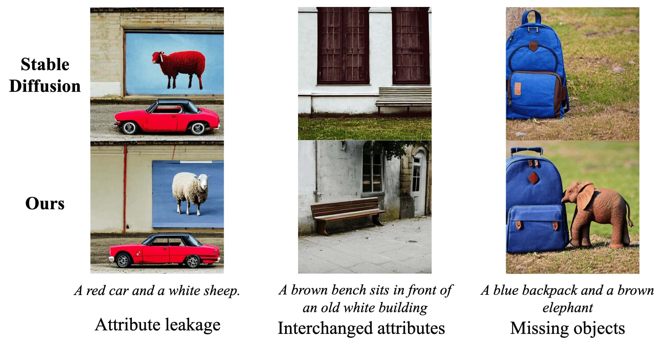
Large-scale T2I models, such as Imagen, DALLE-2, and Stable Diffusion, have systematic weaknesses. For example, current models have a limited ability to compose multiple objects. They also frequently encounter difficulties when generating objects with specified colors and counts, as in the following example:
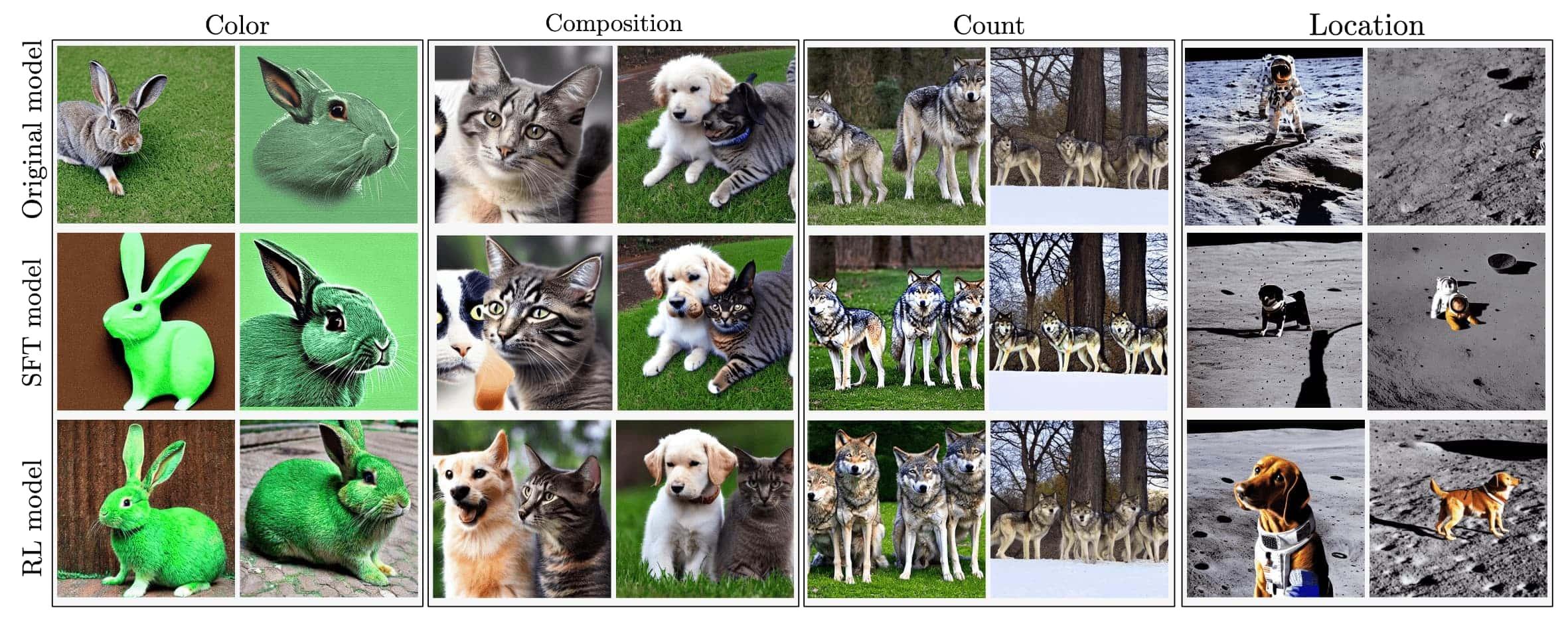
Recently, preference datasets have been studied in fine-tuning diffusion models. Concurrently, DPOK (Fan et al. 2023) and DDPO (Black et al. 2023) proposed to use the preference dataset to train a reward model and then fine-tune diffusion models using reinforcement learning. They showed that RLHF-fine-tuned models can generate images that are better aligned with the input text prompts than the original T2I models.
DDPO (Denoising Diffusion Policy Optimization)
Denoising Diffusion Policy Optimization (DDPO) fine-tuned T2I diffusion models using online RL on $T$-step MDP formulation. They showed that optimizing the expected reward of image output is equivalent to performing policy gradient under some regularity conditions.
Additionally, they proposed the reward model for automated prompt alignment using LLaVA and BERTScore. This reward model is evaluated by BERTScore, which outputs the similarity between the prompt and the VLM description of the generated image:

RL Fine-tuning of Diffusion Models
To apply RL algorithm for fine-tuning, the authors firstly modeled denoising process of T2I diffusion model \(p_\boldsymbol{\theta} (\mathbf{x}_{0:T} \vert \mathbf{z})\) as a $T$-horizon MDP:
\[\begin{aligned} & \mathbf{s}_t = (\mathbf{z}, \mathbf{x}_{T-t}), \quad \;\; \mathbf{a}_t = \mathbf{x}_{T-t-1}, \quad \;\; \rho_0 (\mathbf{s}_0) = \big(p(\mathbf{z}),\mathcal{N}(\mathbf{0},\mathbf{I})\big), \quad\;\; \mathcal{T}(\mathbf{s}_{t+1} \mid \mathbf{s}_t, \mathbf{a}_t) = (\delta_\mathbf{z},\delta_{\mathbf{a}_t}) \\ & R(\mathbf{s}_t, \mathbf{a}_t) = \begin{cases} r_\boldsymbol{\phi}(\mathbf{x}_0, \mathbf{z}) & \text{if } \; t = T-1 \\ 0 & \text{otherwise}. \end{cases}, \quad\;\; \pi_\boldsymbol{\theta} (\mathbf{a}_t \mid \mathbf{s}_t) = p_\boldsymbol{\theta} (\mathbf{x}_{T-t-1} \mid \mathbf{x}_{T-t}, \mathbf{z}), \end{aligned}\]where $r_\boldsymbol{\phi}$ is the reward model trained using human assessment of images, and $\delta$ is the Dirac distribution. Note that the reward is given only at the final step in which the quality of the image at the end of the denoising process. Therefore, the goal of fine-tuning the diffusion models is to maximize the expected reward of the generated images $\mathbf{x}_0$ given the prompt distribution $p(\mathbf{z})$:
\[\max_\boldsymbol{\theta} \mathcal{L}_\texttt{DDPO} (\boldsymbol{\theta}) = \mathbb{E}_{p(\mathbf{z})} \mathbb{E}_{p_\boldsymbol{\theta} (\mathbf{x}_0 \vert \mathbf{z})} \left[ r (\mathbf{x}_0, \mathbf{z}) \right]\]Then, we can show that optimizing the expected reward of image output is equivalent to performing policy gradient under the condition that \(p_\boldsymbol{\theta} (\mathbf{x}_{0:T} \vert \mathbf{z}) r(\mathbf{x}_0, \mathbf{z})\) and \(\nabla_\boldsymbol{\theta} p_\boldsymbol{\theta} (\mathbf{x}_{0:T} \vert \mathbf{z}) r(\mathbf{x}_0, \mathbf{z})\) are continuous function of $\boldsymbol{\theta}$:
\[\nabla_{\boldsymbol{\theta}} \mathbb{E}_{p(\mathbf{z})} \mathbb{E}_{p_\boldsymbol{\theta} (\mathbf{x}_0 \vert \mathbf{z})} [r(\mathbf{x}_0,\mathbf{z})] = \mathbb{E}_{p(\mathbf{z})}\mathbb{E}_{p_\boldsymbol{\theta}(\mathbf{x}_{0:T} \vert \mathbf{z})}\left[- r(\mathbf{x}_0,\mathbf{z}) \sum_{t=1}^{T} \nabla_{\boldsymbol{\theta}}\log p_{\boldsymbol{\theta}}(\mathbf{x}_{t-1} \vert \mathbf{x}_{t},\mathbf{z}) \right] .\]Consequently, we can apply any policy gradient algorithms including PPO to fine-tune the T2I diffusion models.
DPOK (Diffusion Policy Optimization with KL regularization)
Diffusion Policy Optimization with KL regularization (DPOK) combined the KL divergence regularization with respect to the pre-trained diffusion model into the DDPO loss and use it to better align text-to-image objectives. They showed that KL regularization in RL fine-tuning of T2I diffusion is effective in attaining both high reward and aesthetic scores.

RL Fine-tuning with KL divergence
The danger of fine-tuning purely based on the reward model learned from human or AI feedback lies in the potential for the model to overfit to the reward, thereby undervaluing the inherent “skill” of the initial diffusion model more than is justified. To mitigate this issue, similar to InstructGPT, the authors introduced a KL regularizer between the fine-tuned \(p_\boldsymbol{\theta}\) and pre-trained diffusion models $p_\texttt{pre}$:
\[\mathrm{KL} \left(p_\boldsymbol{\theta} (\mathbf{x}_0 \vert \mathbf{z}) \Vert p_\texttt{pre} (\mathbf{x}_0 \vert \mathbf{z}) \right)\]To avoid the intractability of the marginal $p_\boldsymbol{\theta} (\mathbf{x}_0 \vert \mathbf{z})$, this KL divergence is implicitly optimized using the following upper-bound:
\[\require{cancel} \begin{aligned} \mathrm{KL} \left(p_\boldsymbol{\theta} (\mathbf{x}_0 \vert \mathbf{z}) \Vert p_\texttt{pre} (\mathbf{x}_0 \vert \mathbf{z}) \right) & \leq \mathrm{KL} \left(p_\boldsymbol{\theta} (\mathbf{x}_{0:T} \vert \mathbf{z}) \Vert p_\texttt{pre} (\mathbf{x}_{0:T} \vert \mathbf{z}) \right) \\ & = \int p_\boldsymbol{\theta} (\mathbf{x}_{0:T} \vert \mathbf{z}) \times \log \frac{p_\boldsymbol{\theta} (\mathbf{x}_{0:T} \vert \mathbf{z})}{p_\texttt{pre} (\mathbf{x}_{0:T} \vert \mathbf{z})} d \mathbf{x}_{0:T} \\ & = \int p_\boldsymbol{\theta} (\mathbf{x}_{0:T} \vert \mathbf{z}) \left( \cancel{\log \frac{p_\boldsymbol{\theta} (\mathbf{x}_T \vert \mathbf{z})}{p_\texttt{pre} (\mathbf{x}_T \vert \mathbf{z})}} + \sum_{t=1}^T \log \frac{p_\boldsymbol{\theta} (\mathbf{x}_{t-1} \vert \mathbf{x}_t, \mathbf{z})}{p_\texttt{pre} (\mathbf{x}_{t-1} \vert \mathbf{x}_t, \mathbf{z})} \right) d \mathbf{x}_{0:T} & \because p (\mathbf{x}_T \vert \mathbf{z}) \sim \mathcal{N} (\mathbf{0}, \mathbf{I}) \\ & = \sum_{t=1}^T \mathbb{E}_{p_\boldsymbol{\theta} (\mathbf{x}_{t:T} \vert \mathbf{z})} \mathbb{E}_{p_\boldsymbol{\theta} (\mathbf{x}_{0:t-1} \vert \mathbf{x}_{t:T}, \mathbf{z})} \left[ \log \frac{p_\boldsymbol{\theta} (\mathbf{x}_{t-1} \vert \mathbf{x}_t, \mathbf{z})}{p_\texttt{pre} (\mathbf{x}_{t-1} \vert \mathbf{x}_t, \mathbf{z})} \right] \\ & = \sum_{t=1}^T \mathbb{E}_{p_\boldsymbol{\theta} (\mathbf{x}_t \vert \mathbf{z})} \mathbb{E}_{p_\boldsymbol{\theta} (\mathbf{x}_{t-1} \vert \mathbf{x}_t, \mathbf{z})} \left[ \log \frac{p_\boldsymbol{\theta} (\mathbf{x}_{t-1} \vert \mathbf{x}_t, \mathbf{z})}{p_\texttt{pre} (\mathbf{x}_{t-1} \vert \mathbf{x}_t, \mathbf{z})} \right] & \because \textrm{Markov Property} \\ & = \sum_{t=1}^T \mathbb{E}_{p_\boldsymbol{\theta} (\mathbf{x}_t \vert \mathbf{z})} \left[ \mathrm{KL} \left(p_\boldsymbol{\theta} (\mathbf{x}_{t-1} \vert \mathbf{x}_t, \mathbf{z}) \Vert p_\texttt{pre} (\mathbf{x}_{t-1} \vert \mathbf{x}_t, \mathbf{z}) \right) \right] \end{aligned}\]Consequently, the following objective with KL-regularized is referred to as DPOK:
\[\begin{aligned} \mathcal{L}_\texttt{DPOK} (\boldsymbol{\theta}) = - \mathbb{E}_{p(\mathbf{z})} \Bigl[ \alpha \cdot \mathbb{E}_{p_\boldsymbol{\theta} (\mathbf{x}_{0:T} \vert \mathbf{z})} [r (\mathbf{x}_0, \mathbf{z})] + \beta \cdot \sum_{t=1}^T \mathbb{E}_{p_\boldsymbol{\theta} (\mathbf{x}_t \vert \mathbf{z})} \bigl[ \mathrm{KL} \left(p_\boldsymbol{\theta} (\mathbf{x}_{t-1} \vert \mathbf{x}_t, \mathbf{z}) \Vert p_\texttt{pre} (\mathbf{x}_{t-1} \vert \mathbf{x}_t, \mathbf{z}) \right) \bigr] \Bigr] \end{aligned}\]Direct Preference Optimization of Diffusion
DDPO and DPOK necessitate a robust reward model, which demands a substantial dataset of images and extensive human evaluations. Drawing inspiration from the DPO, Diffusion-DPO (Wallace et al. 2023) and D3PO (Yang et al. 2023) used the implicit reward to fine-tune diffusion models directly on the preference dataset.
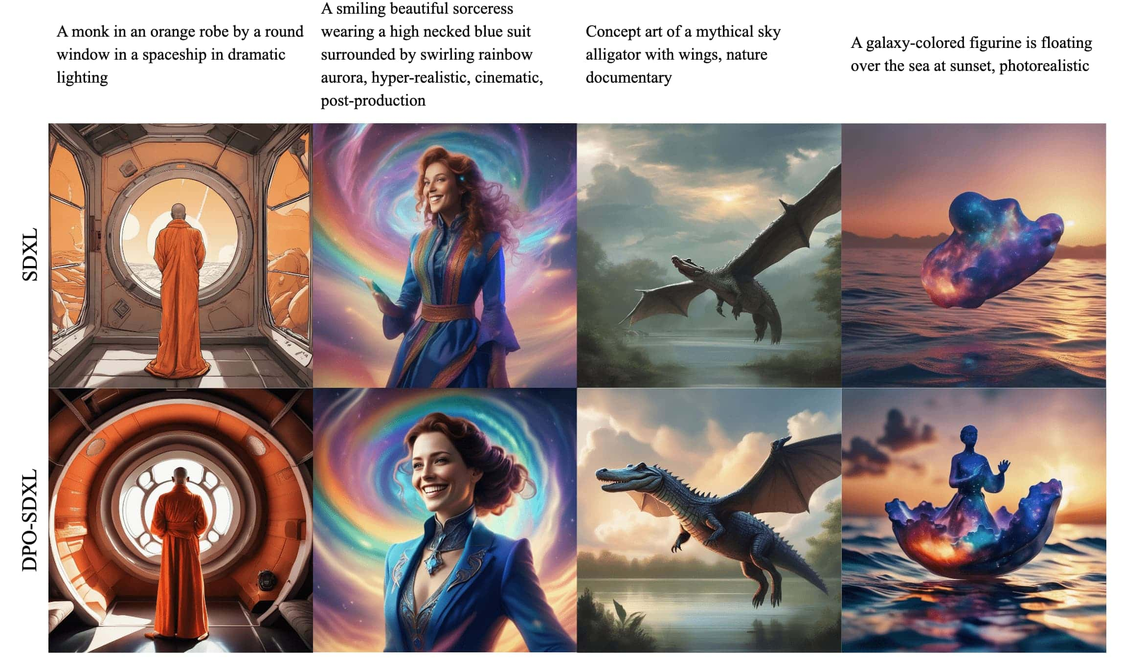
Diffusion-DPO (Diffusion Direct Preference Optimization)
In adapting DPO to T2I diffusion models \(p_\boldsymbol{\theta} (\mathbf{x}_0 \vert \mathbf{z})\), consider a fixed dataset \(\mathcal{D} = \{( \mathbf{z}, \mathbf{x}_0^w, \mathbf{x}_0^l )\}\) where each example contains a prompt $\mathbf{z}$ and a pairs of images generated from a reference model pref with human preference \(\mathbf{x}_0^w \succ \mathbf{x}_0^l\). Then, we can adapt the DPO loss to diffusion models as following:
\[\begin{gathered} \mathcal{L}_\texttt{DPO} (\boldsymbol{\theta}) = - \mathbb{E}_{(\mathbf{x}, \mathbf{y}_w, \mathbf{y}_l) \sim \mathcal{D}} \left[ \log \sigma \left( \beta \cdot \log \frac{\pi_\boldsymbol{\theta} (\mathbf{y}_w \vert \mathbf{x})}{\pi_\texttt{SFT} (\mathbf{y}_w \vert \mathbf{x})} - \beta \cdot \log \frac{\pi_\boldsymbol{\theta} (\mathbf{y}_l \vert \mathbf{x})}{\pi_\texttt{SFT} (\mathbf{y}_l \vert \mathbf{x})} \right) \right] \\ \Big\Downarrow \\ \mathcal{L} (\boldsymbol{\theta}) = - \mathbb{E}_{(\mathbf{z}, \mathbf{x}_0^w, \mathbf{x}_0^l) \sim \mathcal{D}} \left[ \log \sigma \left( \beta \cdot \mathbb{E}_{\begin{aligned} & \mathbf{x}_{1:T}^w \sim p_\boldsymbol{\theta} (\cdot \vert \mathbf{x}_0^w, \mathbf{z}) \\ & \mathbf{x}_{1:T}^l \sim p_\boldsymbol{\theta} (\cdot \vert \mathbf{x}_0^l, \mathbf{z}) \end{aligned}} \left[ \log \frac{p_\boldsymbol{\theta} \left(\mathbf{x}_{0:T}^w \vert \mathbf{z} \right)}{p_\text{ref} \left(\mathbf{x}_{0:T}^w \vert \mathbf{z} \right)} - \log \frac{p_\boldsymbol{\theta} \left(\mathbf{x}_{0:T}^l \vert \mathbf{z} \right)}{p_\text{ref} \left(\mathbf{x}_{0:T}^l \vert \mathbf{z} \right)} \right] \right) \right] \end{gathered}\]Since sampling from \(p_\boldsymbol{\theta} (\mathbf{x}_{1:T} \vert \mathbf{x}_0, \mathbf{z})\) is intractable, we instead utilize forward process $q (\mathbf{x}_{1:T} \vert \mathbf{x}_0)$:
\[\mathcal{L} (\boldsymbol{\theta}) = - \mathbb{E}_{(\mathbf{z}, \mathbf{x}_0^w, \mathbf{x}_0^l) \sim \mathcal{D}} \left[ \log \sigma \left( \beta \cdot \mathbb{E}_{\begin{aligned} & \mathbf{x}_{1:T}^w \sim \color{blue}{q (\cdot \vert \mathbf{x}_0^w, \mathbf{z})} \\ & \mathbf{x}_{1:T}^l \sim \color{blue}{q (\cdot \vert \mathbf{x}_0^l, \mathbf{z})} \end{aligned}} \left[ \log \frac{p_\boldsymbol{\theta} \left(\mathbf{x}_{0:T}^w \vert \mathbf{z} \right)}{p_\text{ref} \left(\mathbf{x}_{0:T}^w \vert \mathbf{z} \right)} - \log \frac{p_\boldsymbol{\theta} \left(\mathbf{x}_{0:T}^l \vert \mathbf{z} \right)}{p_\text{ref} \left(\mathbf{x}_{0:T}^l \vert \mathbf{z} \right)} \right] \right) \right]\]and ELBO by Jensen’s inequality from the convexity of $-\log \sigma$:
\[\begin{aligned} & \mathcal{L} (\boldsymbol{\theta}) \leq - \mathbb{E}_{(\mathbf{z}, \mathbf{x}_0^w, \mathbf{x}_0^l) \sim \mathcal{D}, t \sim U (0, T), \mathbf{x}_{t-1 : t}^w \sim q (\cdot \vert \mathbf{x}_0^w, \mathbf{z}), \mathbf{x}_{t-1 : t}^l \sim q (\cdot \vert \mathbf{x}_0^l, \mathbf{z})} \Biggl[ \\ & \quad \log \sigma \left( \beta \cdot T \cdot \left( \log \frac{p_\boldsymbol{\theta} \left(\mathbf{x}_{t-1}^w \vert \mathbf{x}_t^w, \mathbf{z} \right)}{p_\text{ref} \left(\mathbf{x}_{t-1}^w \vert \mathbf{x}_t^w, \mathbf{z} \right)} - \log \frac{p_\boldsymbol{\theta} \left(\mathbf{x}_{t-1}^l \vert \mathbf{x}_t^l,\mathbf{z} \right)}{p_\text{ref} \left(\mathbf{x}_{t-1}^l \vert \mathbf{x}_t^l, \mathbf{z} \right)} \right) \right) \Biggr] \\ & = - \mathbb{E}_{(\mathbf{z}, \mathbf{x}_0^w, \mathbf{x}_0^l) \sim \mathcal{D}, t \sim U (0, T), \mathbf{x}_t^w \sim q (\cdot \vert \mathbf{x}_0^w, \mathbf{z}), \mathbf{x}_t^l \sim q (\cdot \vert \mathbf{x}_0^l, \mathbf{z})} \Biggl[ \\ & \quad \log \sigma \Bigl( - \beta T ( \\ & \quad + \mathrm{KL} \left(q (\mathbf{x}_{t-1}^w \vert \mathbf{x}_{0, t}^w, \mathbf{z} ) \middle\Vert p_\boldsymbol{\theta} \left(\mathbf{x}_{t-1}^w \vert \mathbf{x}_t^w, \mathbf{z} \right) \right) \\ & \quad - \mathrm{KL} \left(q (\mathbf{x}_{t-1}^w \vert \mathbf{x}_{0, t}^w, \mathbf{z} ) \middle\Vert p_\texttt{ref} \left(\mathbf{x}_{t-1}^w \vert \mathbf{x}_t^w, \mathbf{z} \right) \right) \\ & \quad - \mathrm{KL} \left(q (\mathbf{x}_{t-1}^l \vert \mathbf{x}_{0, t}^l, \mathbf{z} ) \middle\Vert p_\boldsymbol{\theta} \left(\mathbf{x}_{t-1}^l \vert \mathbf{x}_t^l, \mathbf{z} \right) \right) \\ & \quad - \mathrm{KL} \left(q (\mathbf{x}_{t-1}^l \vert \mathbf{x}_{0, t}^l, \mathbf{z} ) \middle\Vert p_\texttt{ref} \left(\mathbf{x}_{t-1}^l \vert \mathbf{x}_t^l, \mathbf{z} \right) \right) \Bigr) \Biggr] \end{aligned}\]Then, from the forward/reverse process we parameterized, it is possible to replace these KL divergences by noise predictions. For example, in DDPM formulation, recall that:
\[\begin{aligned} q (\mathbf{x}_t \vert \mathbf{x}_{t-1}) & = \mathcal{N} \left( \sqrt{ \alpha_t^2 } \mathbf{x}_{t-1}, \sigma_t^2 = \beta_t \mathbf{I} \right) \\ p_\boldsymbol{\theta} (\mathbf{x}_{t-1} \vert \mathbf{x}_t) & = \mathcal{N} (\boldsymbol{\mu}_\boldsymbol{\theta} (\mathbf{x}_t), \sigma_t^2 \mathbf{I}) \\ & \Big\Downarrow \\ q (\mathbf{x}_{t-1} \vert \mathbf{x}_t, \mathbf{x}_0) & = \mathcal{N} \left(\frac{1}{\sqrt{\alpha_t}} \left( \mathbf{x}_t - \frac{1 - \alpha_t}{\sqrt{1 - \bar{\alpha}_t}} \boldsymbol{\epsilon}_t \right), \frac{1 - \bar{\alpha}_{t-1}}{1 - \bar{\alpha}_t} \cdot \beta_t \mathbf{I} \right) \\ \mathrm{KL} (q (\mathbf{x}_{t-1} \vert \mathbf{x}_t, \mathbf{x}_0) \Vert p_\boldsymbol{\theta} (\mathbf{x}_{t-1} \vert \mathbf{x}_t) ) & = \mathbb{E}_{\boldsymbol{x}_0, \boldsymbol{\epsilon}} \left[ \left[\frac{\beta_t^2}{2 \sigma_t^2 \alpha_t\left(1-\bar{\alpha}_t\right)}\left \Vert \boldsymbol{\epsilon}-\boldsymbol{\epsilon}_\theta\left(\mathbf{x}_t, t\right)\right \Vert ^2\right] \right] \end{aligned}\]Consequently, we obtain the final objective called Diffusion-DPO as following:
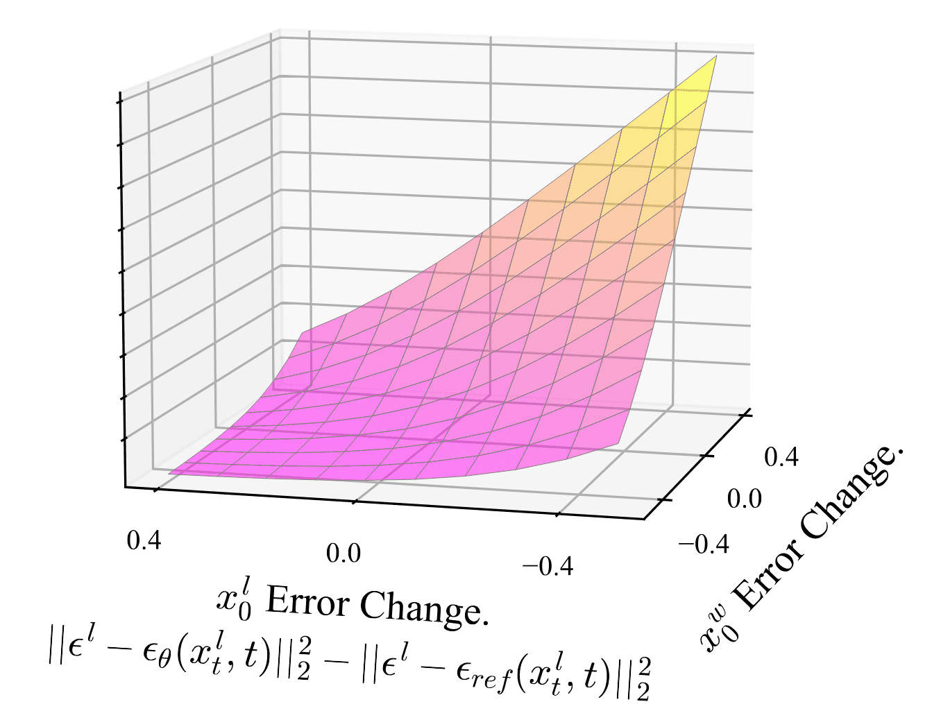
\[\begin{multline*} \mathcal{L}_\texttt{DPO-Diffusion} (\boldsymbol{\theta}) = - \mathbb{E}_{t, \mathbf{z}, \boldsymbol{\epsilon}^w, \boldsymbol{\epsilon}^l} [ \log \sigma ( - \beta T \omega (\lambda_t) \{ ( \Vert \boldsymbol{\epsilon}^w - \boldsymbol{\epsilon}_\boldsymbol{\theta} (\mathbf{x}_t^w, \mathbf{z}, t) \Vert^2 - \Vert \boldsymbol{\epsilon}^w - \boldsymbol{\epsilon}_\texttt{ref} ( \mathbf{x}_t^w, \mathbf{z}, t ) \Vert^2 ) \\ - ( \Vert \boldsymbol{\epsilon}^l - \boldsymbol{\epsilon}_\boldsymbol{\theta} ( \mathbf{x}_t^l, \mathbf{z}, t) \Vert^2 - \Vert \boldsymbol{\epsilon}^l - \boldsymbol{\epsilon}_\texttt{ref} ( \mathbf{x}_t^l, \mathbf{z}, t ) \Vert^2 ) ) \} ] \end{multline*}\]where $\lambda_t$ is a signal-to-noise ratio ($\alpha_t^2 / \sigma_t^2$ in case of DDPM) and $\omega (\lambda_t)$ is a pre-specified weighting function. This loss encourages \(\boldsymbol{\epsilon}_\boldsymbol{\theta}\) to improve more at denoising \(\mathbf{x}_t^w\) than \(\mathbf{x}_t^l\), as visualized in the next figure:
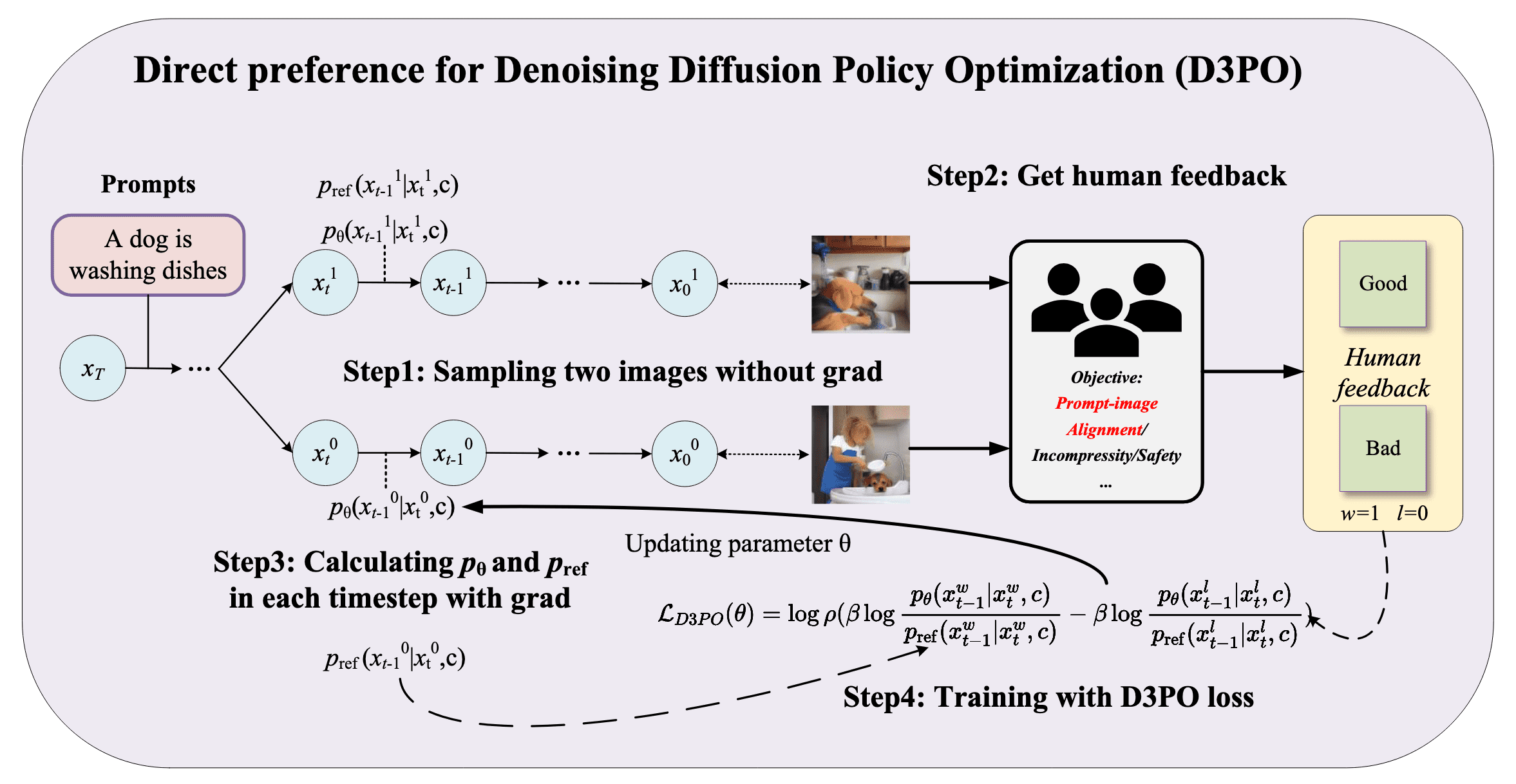
D3PO (Direct Preference for DDPO)
While Diffusion-DPO directly adapts the DPO loss into the formulation of T2I diffusion models, extend the DPO theory to MDP, which allows us to apply the principles to effectively translate human preferences into policy improvements in diffusion models.
DPO for MDP
Again, we define the $T$-step MDP as identical to the DDPO:
\[\begin{aligned} & \mathbf{s}_t = (\mathbf{z}, \mathbf{x}_{T-t}), \quad \;\; \mathbf{a}_t = \mathbf{x}_{T-t-1}, \quad \;\; \rho_0 (\mathbf{s}_0) = \big(p(\mathbf{z}),\mathcal{N}(\mathbf{0},\mathbf{I})\big), \quad\;\; \mathcal{T}(\mathbf{s}_{t+1} \mid \mathbf{s}_t, \mathbf{a}_t) = (\delta_\mathbf{z},\delta_{\mathbf{a}_t}) \\ & \pi_\boldsymbol{\theta} (\mathbf{a}_t \mid \mathbf{s}_t) = p_\boldsymbol{\theta} (\mathbf{x}_{T-t-1} \mid \mathbf{x}_{T-t}, \mathbf{z}) \end{aligned}\]but in contrast, recall that we should formulate the reward as follows in the DPO theory:
\[r (\mathbf{x}, \mathbf{y}) = \beta \cdot \log \frac{\pi_\boldsymbol{\theta} (\mathbf{y} \vert \mathbf{x})}{\pi_\texttt{SFT} (\mathbf{y} \vert \mathbf{x})} + \beta \cdot \log Z (\mathbf{x})\]Consequently, the objective of D3PO is to maximize the expected return instead of the single reward in the DDPO & DPOK, where the reward is given only at the final step in which the quality of the image at the end of the denoising process:
\[\max_\pi \mathbb{E}_{\mathbf{s} \sim d^\pi, \mathbf{a} \sim \pi(\cdot \vert \mathbf{s})} \left[Q^* (\mathbf{s}, \mathbf{a}) \right] - \beta \cdot \mathrm{KL} \left( \pi (\cdot \vert \mathbf{s}) \Vert \pi_\texttt{ref} (\cdot \vert \mathbf{s}) \right)\]And analogous to DPO, we can derive the analytical mapping from optimal state-action values to optimal policies:
\[\begin{aligned} & \max_{\pi} \; \mathbb{E}_{\mathbf{s} \sim d^\pi, \mathbf{a} \sim \pi(\cdot\vert\mathbf{s})}[Q^*(\mathbf{s}, \mathbf{a})] - \beta \cdot \mathrm{KL} \left( \pi (\cdot \vert \mathbf{s}) \Vert \pi_\texttt{ref} (\cdot \vert \mathbf{s}) \right) \\ = & \; \max_\pi \; \mathbb{E}_{\mathbf{s} \sim d^\pi, \mathbf{a} \sim \pi(\cdot\vert\mathbf{s})} \left[ Q^*(\mathbf{s}, \mathbf{a})-\beta \cdot \log\dfrac{\pi(\mathbf{a}\vert\mathbf{s})}{\pi_\texttt{ref}(\mathbf{a}\vert\mathbf{s})} \right] \\ = & \; \min_\pi \; \mathbb{E}_{\mathbf{s} \sim d^\pi, \mathbf{a} \sim \pi(\cdot\vert\mathbf{s})}\left[\log\dfrac{\pi(\mathbf{a}\vert\mathbf{s})}{\pi_\texttt{ref}(\mathbf{a}\vert\mathbf{s})}-\dfrac{1}{\beta}Q^*(\mathbf{s}, \mathbf{a})\right] \\ = & \; \min_\pi \; \mathbb{E}_{\mathbf{s} \sim d^\pi, \mathbf{a} \sim \pi(\cdot\vert\mathbf{s})}\left[\log\dfrac{\pi(\mathbf{a}\vert\mathbf{s})}{ \pi_\texttt{ref}(\mathbf{a}\vert\mathbf{s})\exp \left(\dfrac{1}{\beta} Q^*(\mathbf{s}, \mathbf{a}) \right) = \tilde{\pi}(\mathbf{a}\vert\mathbf{s})} \right]\\ = & \; \min_\pi \; \mathbb{E}_{\mathbf{s} \sim d^\pi}\left[\mathrm{KL} \left( \pi(\cdot\vert\mathbf{s})\Vert \tilde{\pi}(\cdot\vert\mathbf{s}) \right) \right] \end{aligned}\]which gives the mapping:
\[\begin{aligned} & \pi^* (\mathbf{a} \vert \mathbf{s}) = \frac{1}{Z(\mathbf{s})} \pi_\texttt{ref}(\mathbf{a}\vert\mathbf{s})\exp \left(\dfrac{1}{\beta} Q^*(\mathbf{s}, \mathbf{a}) \right) \\ \Rightarrow & \; Q^* (\mathbf{s}, \mathbf{a}) = \beta \cdot \log \frac{\pi^* (\mathbf{a} \vert \mathbf{s})}{\pi_\texttt{ref}(\mathbf{a}\vert\mathbf{s})} - \beta \cdot \log Z (\mathbf{s}) \end{aligned}\]and the preference model:
\[\begin{gathered} p (\tau_w \succ \tau_l) = \sigma \left( Q^* (\mathbf{s}_k^w, \mathbf{a}_k^w) - Q^* (\mathbf{s}_l, \mathbf{a}_l) \right) = \frac{\exp \left( Q^* (\mathbf{s}_k^w, \mathbf{a}_k^w) \right)}{\exp \left( Q^* (\mathbf{s}_k^w, \mathbf{a}_k^w) \right) + \exp \left( Q^* (\mathbf{s}_l, \mathbf{a}_l) \right)} \\ \Big\Downarrow \\ p ((\mathbf{s}_k^w, \mathbf{a}_k^w) \succ (\mathbf{s}_l, \mathbf{a}_l)) = \frac{1}{1 + \exp \left( \beta \cdot \log \dfrac{\pi^* (\mathbf{a}_l \vert \mathbf{s}_l)}{\pi_\texttt{ref} (\mathbf{a}_l \vert \mathbf{s}_l)} - \beta \cdot \log \dfrac{\pi^* (\mathbf{a}_k^w \vert \mathbf{s}_k^w)}{\pi_\texttt{ref} (\mathbf{a}_k^w \vert \mathbf{s}_k^w)} \right)} \end{gathered}\]where \(\tau = \{ \mathbf{s}_k, \mathbf{a}_k, \mathbf{s}_{k+1}, \cdots, \mathbf{s}_T, \mathbf{a}_T\}\). Consequently, our cross-entropy objective becomes:
\[\begin{gathered} \mathcal{L}_\texttt{reward} (\boldsymbol{\theta}) = - \mathbb{E}_{(\mathbf{s}_k, \tau_w, \tau_l) \sim \mathcal{D}} \left[ \log \sigma \left( Q_\boldsymbol{\theta} (\mathbf{s}_k^w, \mathbf{a}_k^w) - Q_\boldsymbol{\theta} (\mathbf{s}_k^l, \mathbf{a}_k^l) \right) \right] \\ \Big\Downarrow \\ \begin{aligned} \mathcal{L}_\texttt{D3PO} (\boldsymbol{\theta}) & = - \mathbb{E}_{(\mathbf{s}_k, \tau_w, \tau_l) \sim \mathcal{D}} \left[ \log \sigma \left( \beta \cdot \log \dfrac{\pi^* (\mathbf{a}_k^w \vert \mathbf{s}_k^w)}{\pi_\texttt{ref} (\mathbf{a}_k^w \vert \mathbf{s}_k^w)} - \beta \cdot \log \dfrac{\pi^* (\mathbf{a}_k^l \vert \mathbf{s}_k^l)}{\pi_\texttt{ref} (\mathbf{a}_k^l \vert \mathbf{s}_k^l)} \right) \right] \\ & = - \mathbb{E}_{\mathbf{z}, t} \left[ \log \sigma \left( \beta \cdot \log \dfrac{p_\boldsymbol{\theta} (\mathbf{x}_{t-1}^w \vert \mathbf{x}_t^w, \mathbf{z})}{p_\texttt{ref} (\mathbf{x}_{t-1}^w \vert \mathbf{x}_t^w, \mathbf{z})} - \beta \cdot \log \dfrac{p_\boldsymbol{\theta} (\mathbf{x}_{t-1}^l \vert \mathbf{x}_t^l, \mathbf{z})}{p_\texttt{ref} (\mathbf{x}_{t-1}^l \vert \mathbf{x}_t^l, \mathbf{z})} \right) \right] \\ \end{aligned} \end{gathered}\]
DCO (Direct Consistency Optimization)
The generation quality of fine-tuning based T2I personalization methods is shown to be heavily dependent on the model’s fitness. For example, the model suffers from image-text alignment when the model overfits to few images used for fine-tuning, making it difficult to generate images with varying attributes around the subject. On the other hand, the model cannot generate consistent subject images when the model underfits.
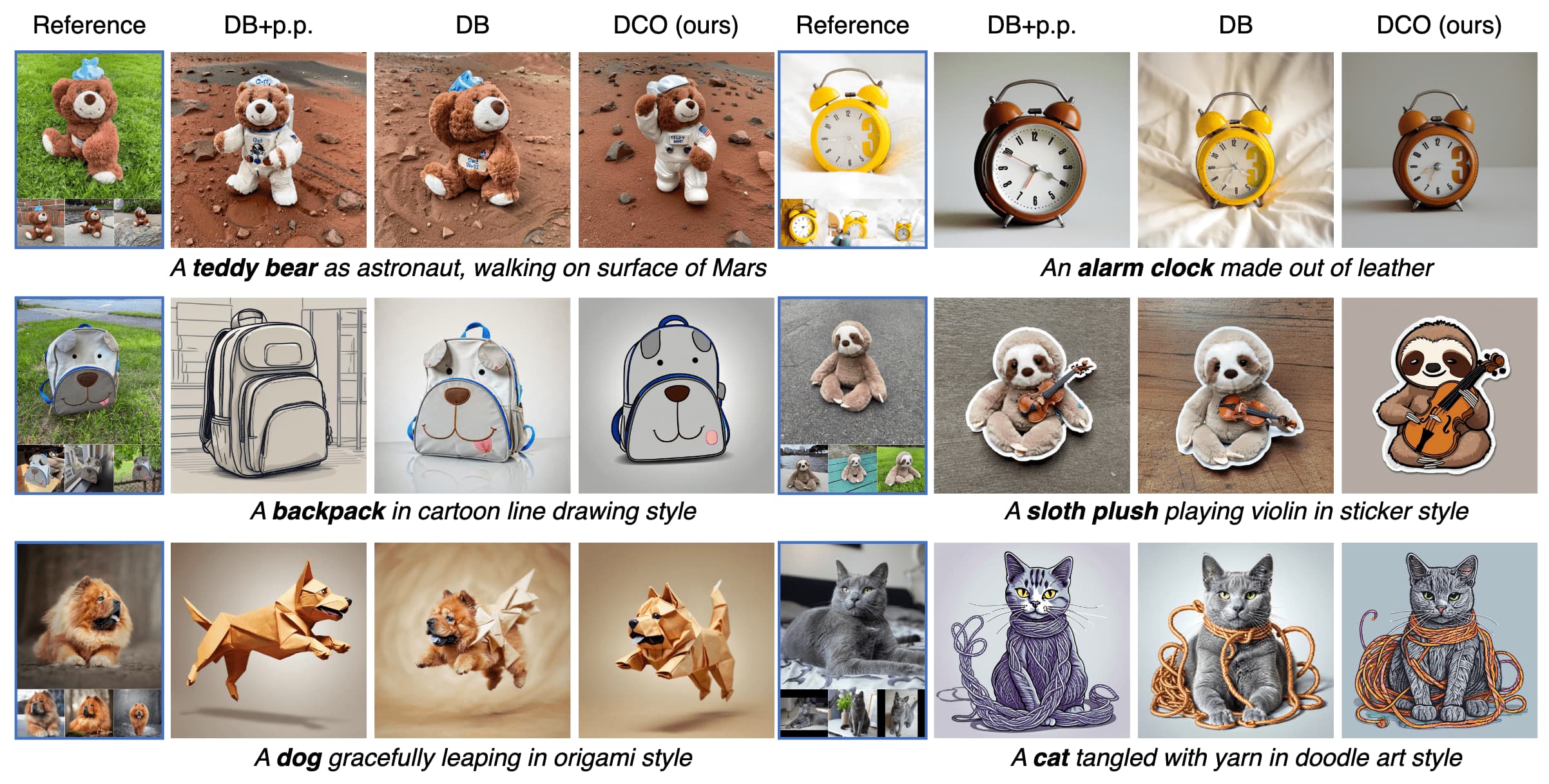
Direct Consistency Optimization (DCO) proposed by Lee et al. 2024 is the first work that used DPO loss for consistency as a reward function for T2I personalization, or few-shot fine-tuning of T2I diffusion models, instead of the human preference.
DCO Reward
Suppose that the reward model $r(\mathbf{x}, \mathbf{z})$ is a reward function that measures the consistency between image $\mathbf{x}$ and reference images, given the relationship between the prompt $\mathbf{z}$ and those of reference images. Then, the DPO objective can be re-written as:
\[\max_\boldsymbol{\theta} \; \mathbb{E}_{\mathbf{z}, \mathbf{x} \sim p_\boldsymbol{\theta} (\cdot \vert \mathbf{z})} \left[ r (\mathbf{x}, \mathbf{z} ) \right] - \beta \cdot \mathrm{KL} \left(p_\boldsymbol{\theta} (\cdot \vert \mathbf{z}) \middle\Vert p_\texttt{ref} (\cdot \vert \mathbf{z}) \right)\]Since \(p_\boldsymbol{\theta} (\mathbf{x}_0 \vert \mathbf{z})\) is intractable, DCO considered the reward \(\hat{r}( \mathbf{x}_{0:T}, \mathbf{z})\) on the diffusion path \(\mathbf{x}_{0:T}\) and re-define the reward by marginalizing over all diffusion path:
\[r(\mathbf{x}_0, \mathbf{z}) = \mathbb{E}_{p_\boldsymbol{\theta} (\mathbf{x}_{1:T} \vert \mathbf{x}_0, \mathbf{z})} \left[ \hat{r} (\mathbf{x}_{0:T}, \mathbf{z}) \right]\]and the lower bound of the DPO objective:
\[\begin{aligned} & \max_\boldsymbol{\theta} \; \mathbb{E}_{\mathbf{z}, \mathbf{x} \sim p_\boldsymbol{\theta} (\cdot \vert \mathbf{z})} \left[ r (\mathbf{x}, \mathbf{z} ) \right] - \beta \cdot \mathrm{KL} \left(p_\boldsymbol{\theta} (\cdot \vert \mathbf{z}) \middle\Vert p_\texttt{ref} (\cdot \vert \mathbf{z}) \right) \\ \geq & \max_\boldsymbol{\theta} \; \mathbb{E}_{\mathbf{z}, \mathbf{x} \sim p_\boldsymbol{\theta} (\cdot \vert \mathbf{z})} \left[ \hat{r} (\mathbf{x}_{0:T}, \mathbf{z} ) \right] - \beta \cdot \mathrm{KL} \left(p_\boldsymbol{\theta} (\mathbf{x}_{0:T} \vert \mathbf{z}) \middle\Vert p_\texttt{ref} (\mathbf{x}_{0:T} \vert \mathbf{z}) \right) \\ & \because \mathrm{KL} \left( q (\mathbf{x}_0) \middle\Vert p (\mathbf{x}_0) \right) \leq \mathrm{KL} \left( q (\mathbf{x}_{0:T}) \middle\Vert p (\mathbf{x}_{0:T}) \right) \end{aligned}\]Again, the closed-form solution to this optimization problem gives the analytical analytical mapping from reward functions to optimal models:
\[p_\boldsymbol{\theta} (\mathbf{x}_{0:T} \vert \mathbf{z}) = \frac{1}{Z(\mathbf{z})} p_\texttt{ref} (\mathbf{x}_{0:T} \vert \mathbf{z}) \exp \left( \frac{1}{\beta} \hat{r} (\mathbf{x}_{0:T}, \mathbf{z}) \right)\]Therefore, the DCO reward is defined as follows:
\[\begin{aligned} & \texttt{DPO: } r (\mathbf{x}, \mathbf{y}) = \beta \cdot \log \frac{\pi_\boldsymbol{\theta} (\mathbf{y} \vert \mathbf{x})}{\pi_\texttt{SFT} (\mathbf{y} \vert \mathbf{x})} + \beta \cdot \log Z (\mathbf{x}) \\ & \texttt{DCO: } r (\mathbf{x}_0, \mathbf{z}) = \begin{aligned}[t] & \mathbb{E}_{\mathbf{x}_{1:T} \sim p_\boldsymbol{\theta} (\cdot \vert \mathbf{x}_0), \mathbf{z}} \left[ \hat{r} (\mathbf{x}_{0:T}, \mathbf{z}) \right] = \mathbb{E}_{\mathbf{x}_{1:T} \sim p_\boldsymbol{\theta} (\cdot \vert \mathbf{x}_0), \mathbf{z}} \left[ \beta \cdot \log \frac{p_\boldsymbol{\theta} (\mathbf{x}_{0:T} \vert \mathbf{z})}{p_\texttt{ref} (\mathbf{x}_{0:T} \vert \mathbf{z})} \right] + \beta \cdot \log Z (\mathbf{z}) \\ & \text{where } \hat{r} (\mathbf{x}_{0:T}, \mathbf{z}) = \beta \cdot \log \frac{p_\boldsymbol{\theta} (\mathbf{x}_{0:T} \vert \mathbf{z})}{p_\texttt{ref} (\mathbf{x}_{0:T} \vert \mathbf{z})} + \beta \cdot \log Z (\mathbf{z}) \end{aligned} \end{aligned}\]DCO Loss
Similar to Diffusion-DPO, the DCO loss also utilized the ELBO by forward process $q$:
\[\begin{aligned} r(\mathbf{x}_0,\mathbf{z}) / \beta &\approx \mathbb{E}_{q(\mathbf{x}_{1:T} \vert \mathbf{x}_0)}\left[ \log \frac{p_\boldsymbol{\theta}(\mathbf{x}_{0:T} \vert \mathbf{z})}{p_\texttt{ref}(\mathbf{x}_{0:T} \vert \mathbf{z})}\right] \\ &=\mathbb{E}_{q(\mathbf{x}_{1:T} \vert \mathbf{x}_0)} \left[ \sum_{t=1}^T \log \frac{p_\boldsymbol{\theta}(\mathbf{x}_{t-1} \vert \mathbf{x}_{t},\mathbf{z})}{p_\texttt{ref}(\mathbf{x}_{t-1}\mathbf{x}_{t},\mathbf{z})} \right]\\ &=\mathbb{E}_{q(\mathbf{x}_{1:T} \vert \mathbf{x}_0)}\left[ \sum_{t=1}^T \log \frac{p_\boldsymbol{\theta}(\mathbf{x}_{t-1} \vert\mathbf{x}_{t},\mathbf{z})}{q(\mathbf{x}_{t-1}\vert\mathbf{x}_t, \mathbf{x}_0)}- \sum_{t=1}^T\log\frac{p_\texttt{ref}(\mathbf{x}_{t-1} \vert \mathbf{x}_{t},\mathbf{z})}{q(\mathbf{x}_{t-1} \vert \mathbf{x}_t, \mathbf{x}_0)} \right]\\ &=\sum_{t=1}^T \mathbb{E}_{q(\mathbf{x}_t \vert \mathbf{x}_0)}\left[ -\mathrm{KL}(q(\mathbf{x}_t \vert \mathbf{x}_{t-1},\mathbf{x}_0) \Vert p_\boldsymbol{\theta}(\mathbf{x}_{t-1} \vert \mathbf{x}_t,\mathbf{z})) + \mathrm{KL}(q(\mathbf{x}_t \vert \mathbf{x}_{t-1},\mathbf{x}_0) \Vert p_\texttt{ref}(\mathbf{x}_{t-1} \vert \mathbf{x}_t,\mathbf{z}))\right]\\ &=\mathbb{E}_{\boldsymbol{\epsilon}\sim\mathcal{N}(\mathbf{0},\mathbf{I}), t\sim\mathcal{U}[0,T]}\left[-T \cdot \omega(t) \cdot \left( \Vert \boldsymbol{\epsilon}_\boldsymbol{\theta}(\mathbf{x}_t;\mathbf{z},t) - \boldsymbol{\epsilon}\Vert_2^2 - \Vert \boldsymbol{\epsilon}_\texttt{ref}(\mathbf{x}_t;\mathbf{z},t) - \boldsymbol{\epsilon}\Vert_2^2 \right)\right] \end{aligned}\]and Jensen’s inequality from the concavity of $\log$:
\[\begin{aligned} & \min_\boldsymbol{\theta} \; \mathbb{E}_{(\mathbf{x}_0, \mathbf{z}) \sim \mathcal{D}} \left[ - \log \sigma ( r( \mathbf{x}_0, \mathbf{z}) ) \right] \\ \leq & \; \min_\boldsymbol{\theta} \underbrace{\mathbb{E}_{(\mathbf{x}_0, \mathbf{z}) \sim \mathcal{D}, \boldsymbol{\epsilon}\sim\mathcal{N}(\mathbf{0},\mathbf{I}), t\sim\mathcal{U}[0,T]} \left[ - \log \sigma \left( - \beta \cdot T \cdot \omega(t) \cdot \left( \Vert \boldsymbol{\epsilon}_\boldsymbol{\theta}(\mathbf{x}_t;\mathbf{z},t) - \boldsymbol{\epsilon}\Vert_2^2 - \Vert \boldsymbol{\epsilon}_\texttt{ref}(\mathbf{x}_t;\mathbf{z},t) - \boldsymbol{\epsilon}\Vert_2^2 \right) \right) \right] }_{\mathcal{L}_\texttt{DCO} (\boldsymbol{\theta})} \end{aligned}\]Therefore, the DPO loss is defined as follows:
\[\mathcal{L}_\texttt{DCO} (\boldsymbol{\theta}) = \mathbb{E}_{(\mathbf{x}_0, \mathbf{z}) \sim \mathcal{D}, \boldsymbol{\epsilon}\sim\mathcal{N}(\mathbf{0},\mathbf{I}), t\sim\mathcal{U}[0,T]} \left[ - \log \sigma \left( - \beta \cdot T \cdot \omega(t) \cdot \left( \Vert \boldsymbol{\epsilon}_\boldsymbol{\theta}(\mathbf{x}_t;\mathbf{z},t) - \boldsymbol{\epsilon}\Vert_2^2 - \Vert \boldsymbol{\epsilon}_\texttt{ref}(\mathbf{x}_t;\mathbf{z},t) - \boldsymbol{\epsilon}\Vert_2^2 \right) \right) \right]\]Since DCO directly regularizes the KL divergence with respect to the samples in references $\mathcal{D}$, it eliminates the need for additional regularizations when fine-tuning T2I models that are used to avoid some issues such as language drift and reduced output diversity. As a result, DCO is free from the trade-offs induced by such regularizations, such as the additional dataset besides the references $\mathcal{D}$.
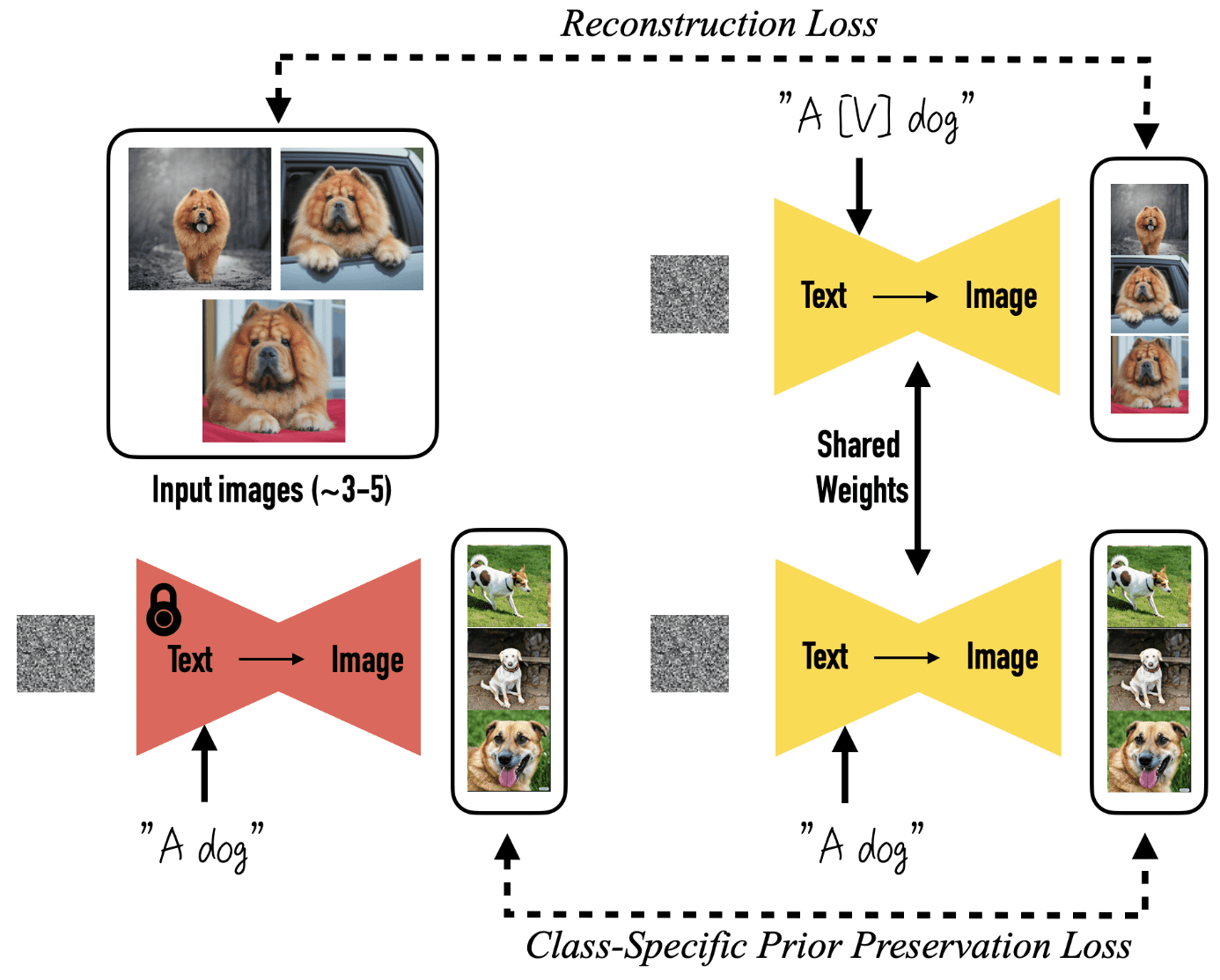
For example, prior preservation loss of DreamBooth:
\[\mathbb{E}_{\mathbf{x}, \mathbf{c}, \boldsymbol{\epsilon}, \boldsymbol{\epsilon}^\prime, t} [w_t \Vert \hat{\mathbf{x}}_\theta (\alpha_t \mathbf{x} + \sigma_t \boldsymbol{\epsilon}, \mathbf{c}) − \mathbf{x} \Vert_2^2 + \lambda w_{t^\prime} \Vert \hat{\mathbf{x}}_\theta (\alpha_{t^\prime} \mathbf{x}_{\mathrm{pr}} + \sigma_{t^\prime} \boldsymbol{\epsilon}^\prime, \mathbf{c}_{\mathrm{pr}}) − \mathbf{x}_{\mathrm{pr}} \Vert_2^2]\]enhances compositional capability but is applied to auxiliary samples, often leading to undesirable model shifts that significantly loses consistency, as illustrated in the second column of $\mathbf{Fig\ 12}$.
Gradient Analysis
Note that the gradient of DCO loss is given as follows:
\[\begin{gathered} \nabla_\boldsymbol{\theta} \mathcal{L}_\texttt{DCO} (\boldsymbol{\theta}) \propto (1 - \sigma (d_t)) \nabla_{\boldsymbol{\theta}} \Vert \boldsymbol{\epsilon}_\boldsymbol{\theta}(\mathbf{x}_t;\mathbf{z},t) - \boldsymbol{\epsilon} \Vert_2^2 \\ \text{ where } d_t = - \beta \cdot T \cdot \left( \Vert \boldsymbol{\epsilon}_\boldsymbol{\theta}(\mathbf{x}_t;\mathbf{z},t) - \boldsymbol{\epsilon} \Vert_2^2 - \Vert \boldsymbol{\epsilon}_\texttt{ref} (\mathbf{x}_t;\mathbf{z},t) - \boldsymbol{\epsilon} \Vert_2^2 \right) \end{gathered}\]This is identical to the gradient of DDPM loss except the scaling factor $(1 - \sigma (d_t))$, which measures the incorrect reward modeling. In other words, DCO loss implicitly performs an adaptive learning rate scheduling for each timestep $t$ by computing deviation from the pretrained model.
Reward Guidance
The presence of consistency reward can be utilized for a guidance method that balances subject consistency and textual alignment. For timestep $t$, define:
\[\begin{gathered} r_t (\mathbf{x}_t, \mathbf{z}) := \beta \log \frac{p_\boldsymbol{\theta} (\mathbf{x}_{t-1} \vert \mathbf{x}_t, \mathbf{z})}{p_\texttt{ref} (\mathbf{x}_{t-1} \vert \mathbf{x}_t, \mathbf{z})} \\ \text{ where } r (\mathbf{x}, \mathbf{z}) = T \cdot \mathbb{E}_{t \sim \mathcal{U}[0, T]} \left[r_t (\mathbf{x}_t, \mathbf{z})\right] \end{gathered}\]Then, the score function of $r_t (\mathbf{x}_t, \mathbf{z})$ is given by:
\[\begin{aligned} \nabla r_t (\mathbf{x}_t, \mathbf{c}) & \propto \nabla \log p_\boldsymbol{\theta} (\mathbf{x}_t \vert \mathbf{z}) - \nabla \log p_\texttt{ref} (\mathbf{x}_t \vert \mathbf{z}) \\ & \propto \boldsymbol{\epsilon}_\boldsymbol{\theta}(\mathbf{x}_t;\mathbf{z},t) - \boldsymbol{\epsilon}_\texttt{ref} (\mathbf{x}_t;\mathbf{z},t) \end{aligned}\]Consequently, by adding this reward guidance that indicates the amount of change from pretrained distribution with scale \(\omega_\texttt{rg}\), the resultant noise estimation of classifier-free guidance (CFG) based T2I model is given as follows:
\[\begin{aligned} \hat{\boldsymbol{\epsilon}}\left(\mathbf{x}_t ; \mathbf{z}, t\right) & = \omega_{\texttt{rg}}\left(\boldsymbol{\epsilon}_\theta\left(\mathbf{x}_t ; \mathbf{z}, t\right)-\boldsymbol{\epsilon}_\texttt{ref} \left(\mathbf{x}_t ; \mathbf{z}, t\right)\right) \\ & + \underbrace{\omega_{\texttt{text}}\left(\boldsymbol{\epsilon}_\texttt{ref} \left(\mathbf{x}_t ; \mathbf{z}, t\right)-\boldsymbol{\epsilon}_\texttt{ref} \left(\mathbf{x}_t; \varnothing, t\right)\right)+\boldsymbol{\epsilon}_\texttt{ref} \left(\mathbf{x}_t; \varnothing, t\right)}_{\textrm{CFG estimator}} \end{aligned}\]where $\omega_\texttt{text}$ is a CFG parameter controlling the prompt fidelity.
References
[1] Christiano et al. “Deep Reinforcement Learning from Human Preferences”, NeurIPS 2017
[2] Ouyang et al. “Training language models to follow instructions with human feedback”, NeurIPS 2022
[3] Rafailov et al. “Direct Preference Optimization: Your Language Model is Secretly a Reward Model”, NeurIPS 2023
[4] Fan et al., “DPOK: Reinforcement Learning for Fine-tuning Text-to-Image Diffusion Models”, NeurIPS 2023
[5] Black et al., “DDPO: Training Diffusion Models with Reinforcement Learning”, ICLR 2024
[6] Wallace et al. “Diffusion Model Alignment Using Direct Preference Optimization”, arXiv preprint arXiv:2311.12908
[7] Yang et al., “D3PO: Using Human Feedback to Fine-tune Diffusion Models without Any Reward Model”, CVPR 2024
[8] Lee et al. “Direct Consistency Optimization for Compositional Text-to-Image Personalization”, arXiv preprint arXiv:2402.12004

Leave a comment