
[Robotics] Spatial Descriptions and Transformations
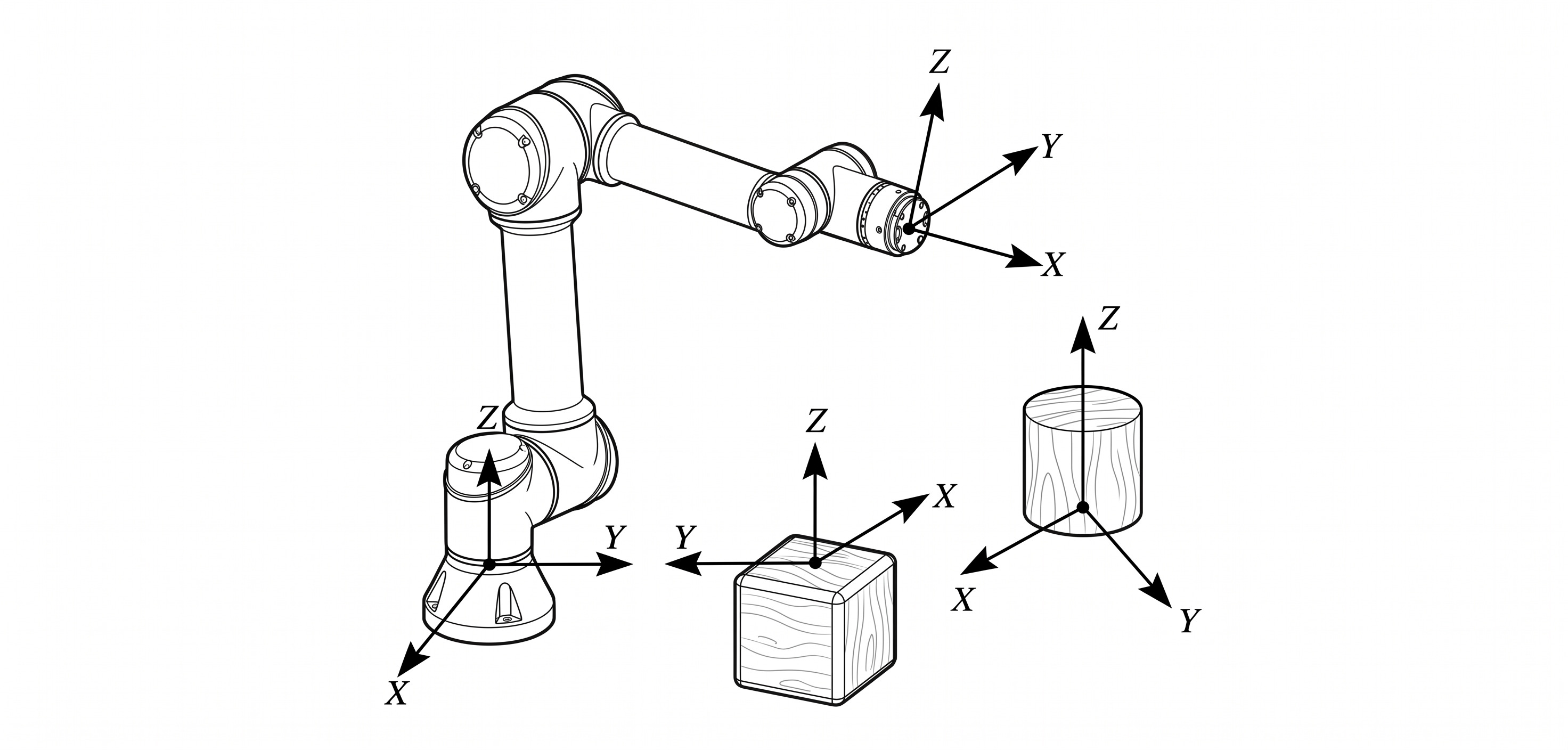
Robotic manipulation, by its very nature, involves the controlled motion of rigid bodies such as links of a manipulator, grasped tools, parts, and objects in the workcell, via three-dimensional space. Before we can describe forward kinematics, plan a trajectory, or compute a Jacobian, we must first agree on a precise mathematical language for where a body is and how it is oriented. This post develops that language: the algebra of positions, orientations, coordinate frames, and the rigid transformations that map between them.
Position
Once a Cartesian coordinate system $\{A\}$ is established, any point $P$ in space can be located by a $3 \times 1$ position vector. Because we will define many coordinate systems beyond the universe frame, every vector must be tagged with information identifying the frame in which it is expressed. We will write a leading superscript indicating that frame:
\[{}^A\mathbf{P} = \begin{bmatrix} p_x \\ p_y \\ p_z \end{bmatrix}\]The components $p_x, p_y, p_z$ are the signed distances along the principal axes $\hat{X}_A, \hat{Y}_A, \hat{Z}_A$ of $\{A\}$; equivalently, they are the projections of $\mathbf{P}$ onto those axes. We adopt right-handed coordinate systems throughout.
A position vector ${}^A\mathbf{P} \in \mathbb{R}^3$ is the ordered triple of signed projections of a point $P$ onto the orthonormal axes of a Cartesian coordinate system $\{ A \}$.
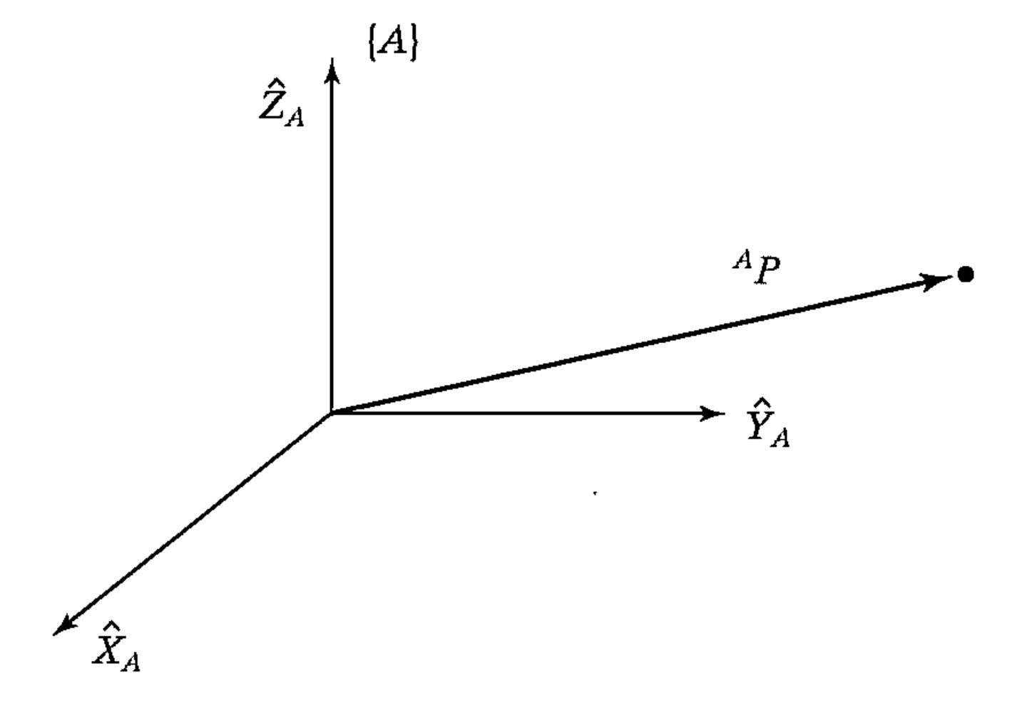
It is essential to remember that the geometric point $P$ is invariant with respect to the choice of frame, while the coordinates assigned to represent it are frame-dependent. Spong and coauthors emphasize this distinction by warning the reader to keep separate the geometric entity $P$ from any coordinate vector that represents it. A direct consequence is that an expression such as ${}^A\mathbf{P} + {}^B\mathbf{Q}$ is geometrically meaningless: vectors expressed in different coordinate frames may not be added.
Orientation
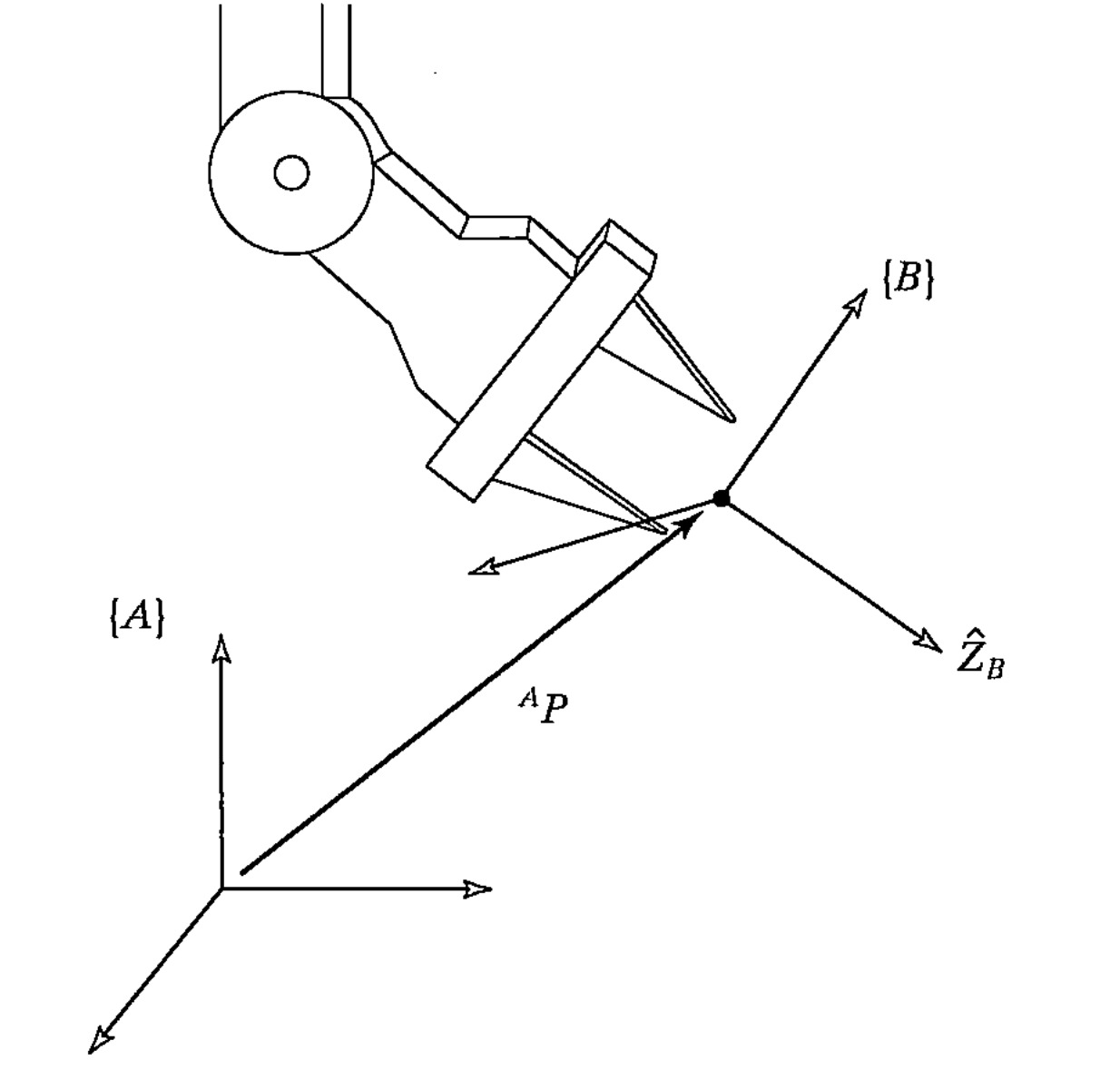
Specifying the position of a body alone does not pin it down in space. A wrench lying on a table may have its centroid at one fixed location yet be oriented in arbitrarily many ways. To describe the orientation of a rigid body, we rigidly attach a coordinate system $\{B\}$ to the body and describe that frame relative to a reference frame $\{A\}$.
Rotation Matrices
Let the unit vectors along the principal axes of $\{B\}$ be $\hat{X}_B, \hat{Y}_B, \hat{Z}_B$. Expressing each in $\{A\}$ gives three vectors ${}^A\hat{X}_B$, ${}^A\hat{Y}_B$, ${}^A\hat{Z}_B$. Stacking them as columns yields the rotation matrix of $\{B\}$ relative to $\{A\}$:
\[{}^A_B R = \begin{bmatrix} {}^A\hat{X}_B & {}^A\hat{Y}_B & {}^A\hat{Z}_B \end{bmatrix} = \begin{bmatrix} r_{11} & r_{12} & r_{13} \\\\ r_{21} & r_{22} & r_{23} \\\\ r_{31} & r_{32} & r_{33} \end{bmatrix}.\]Change of Basis
This column form is not an arbitrary choice; it is forced on us once we insist that the geometric vector $\mathbf{P}$ be invariant under the choice of frame. A coordinate vector ${}^B\mathbf{P} = (p_x^B, p_y^B, p_z^B)^T$ is, by definition, the list of coefficients that expresses $\mathbf{P}$ as a linear combination of the basis vectors of $\{B\}$:
\[\mathbf{P} = p_x^B \, \hat{X}_B + p_y^B \, \hat{Y}_B + p_z^B \, \hat{Z}_B.\]The point $\mathbf{P}$ does not change when we describe it in $\{A\}$, but only its representation does. Each basis vector of $\{B\}$ is itself a geometric arrow, and its coordinates in $\{A\}$ are obtained as follows. Because the axes of $\{A\}$ form an orthonormal basis of $\mathbb{R}^3$, the unit vector $\hat{X}_B$ admits a unique expansion
\[\hat{X}_B \;=\; a_1 \, \hat{X}_A + a_2 \, \hat{Y}_A + a_3 \, \hat{Z}_A.\]Taking the dot product of both sides with \(\hat{X}_i^A\) and invoking orthonormality \(\hat{X}_i^A \cdot \hat{X}_j^A = \delta_{ij}\) isolates the coefficients,
\[a_i \;=\; \hat{X}_B \cdot \hat{X}_i^A,\]so the coordinate triple of $\hat{X}_B$ in $\{A\}$ is
\[{}^A\hat{X}_B \;=\; \begin{bmatrix} \hat{X}_B \cdot \hat{X}_A \\\\ \hat{X}_B \cdot \hat{Y}_A \\\\ \hat{X}_B \cdot \hat{Z}_A \end{bmatrix},\]and analogously for ${}^A\hat{Y}_B$ and ${}^A\hat{Z}_B$. Each entry is the inner product of two unit vectors and therefore equals the cosine of the angle between them, already foreshadowing the direction-cosine identity that will appear shortly. Reading the identity above component-wise in $\{A\}$,
\[{}^A\mathbf{P} \;=\; p_x^B \cdot {}^A\hat{X}_B \;+\; p_y^B \cdot {}^A\hat{Y}_B \;+\; p_z^B \cdot {}^A\hat{Z}_B,\]and the right-hand side is exactly a matrix-vector product:
\[{}^A\mathbf{P} \;=\; \begin{bmatrix} {}^A\hat{X}_B & {}^A\hat{Y}_B & {}^A\hat{Z}_B \end{bmatrix} \begin{bmatrix} p_x^B \\\\ p_y^B \\\\ p_z^B \end{bmatrix} \;=\; {}^A_B R \; {}^B\mathbf{P}.\]Any other choice of columns would make the same geometric vector have inconsistent coordinates in the two frames, so the column-stacked definition of ${}^A_B R$ is the unique matrix that maps coordinates in $\{B\}$ to coordinates in $\{A\}$.
Each scalar entry $r_{ij}$ is the cosine of the angle between an axis of $\{B\}$ and an axis of $\{A\}$, which is why the entries are often called direction cosines:
\[{}^A_B R = \begin{bmatrix} \hat{X}_B \cdot \hat{X}_A & \hat{Y}_B \cdot \hat{X}_A & \hat{Z}_B \cdot \hat{X}_A \\\\ \hat{X}_B \cdot \hat{Y}_A & \hat{Y}_B \cdot \hat{Y}_A & \hat{Z}_B \cdot \hat{Y}_A \\\\ \hat{X}_B \cdot \hat{Z}_A & \hat{Y}_B \cdot \hat{Z}_A & \hat{Z}_B \cdot \hat{Z}_A \end{bmatrix}.\]Inspecting this expression reveals that the rows of ${}^A_B R$ are the unit axes of $\{A\}$ expressed in $\{B\}$. Hence ${}^B_A R$, the rotation matrix describing $\{A\}$ relative to $\{B\}$, equals the transpose of ${}^A_B R$:
\[{}^B_A R = {}^A_B R^T.\]Rotations about a single principal axis admit particularly simple closed forms. A rotation by $\theta$ about $\hat{Z}$ (positive sense by the right-hand rule) is $$ R_z(\theta) = \begin{bmatrix} \cos\theta & -\sin\theta & 0 \\ \sin\theta & \cos\theta & 0 \\ 0 & 0 & 1 \end{bmatrix}. $$ Similarly, rotations about $\hat{X}$ and $\hat{Y}$ are $$ \begin{aligned} R_x(\theta) &= \begin{bmatrix} 1 & 0 & 0 \\ 0 & \cos\theta & -\sin\theta \\ 0 & \sin\theta & \cos\theta \end{bmatrix}, \\[4pt] R_y(\theta) &= \begin{bmatrix} \cos\theta & 0 & \sin\theta \\ 0 & 1 & 0 \\ -\sin\theta & 0 & \cos\theta \end{bmatrix}. \end{aligned} $$ These three matrices, collectively called the basic (or elementary) rotation matrices, satisfy the natural identities $R_a(0) = I$, $R_a(\theta) R_a(\phi) = R_a(\theta + \phi)$, and $R_a(\theta)^{-1} = R_a(-\theta)$ for $a \in \{x, y, z\}$.
Properties and SO(3)
The columns of ${}^A_B R$ are unit-length and mutually orthogonal, which immediately implies
\[{}^A_B R^T \, {}^A_B R = I_3, \quad \text{and therefore} \quad {}^A_B R^{-1} = {}^A_B R^T.\]Such matrices are called orthonormal (or equivalently orthogonal) matrices. Among the orthonormal matrices, the determinant takes the value $\pm 1$. We restrict attention to proper orthonormal matrices, those with $\det R = +1$, which correspond to orientations of right-handed coordinate frames.
The special orthogonal group of order 3 is $$ SO(3) := \{ R \in \mathbb{R}^{3 \times 3} : R^T R = I_3 \text{ and } \det R = +1 \}. $$ Equipped with matrix multiplication as the group operation, $SO(3)$ forms a (non-abelian) Lie group whose elements represent all admissible orientations of a rigid body in three-dimensional space. The analogous group in the plane is $SO(2)$.
Every $R \in SO(n)$ for $n \in \{2, 3\}$ satisfies:
- $R^{-1} = R^T \in SO(n)$.
- Columns (and rows) of $R$ are mutually orthogonal unit vectors.
- $\det R = +1$.
- The product of two rotation matrices is a rotation matrix.
- Matrix multiplication is associative but, for $n = 3$, not commutative in general.
The nine entries $r_{ij}$ are therefore constrained by six independent equations: 3 unit-length constraints and 3 orthogonality constraints
\[\|\hat{X}\| = \|\hat{Y}\| = \|\hat{Z}\| = 1, \quad \hat{X} \cdot \hat{Y} = \hat{X} \cdot \hat{Z} = \hat{Y} \cdot \hat{Z} = 0,\]leaving three independent degrees of freedom. This matches the kinematic intuition that a rigid body in 3D has exactly three rotational degrees of freedom.
Use Cases
A single rotation matrix admits multiple interpretations, and pinning each one down explicitly removes much of the confusion that surrounds rigid-body computation. Namely, we may distinguish three logically distinct uses of an element $R \in SO(3)$. Although the underlying matrix algebra is the same in each case, the geometric meaning differs sharply, and it is exactly this distinction that separates the passive (change-of-coordinates) and active (operator) views of a rotation.
Let $R \in SO(3)$. Then $R$ admits three equivalent geometrical meanings:
- Representation of an orientation. $R = {}^A_B R$ describes the orientation of a frame $\{ B \}$ relative to a reference frame $\{ A \}$. Its columns are the direction cosines of the body axes of $\{ B \}$ expressed in $\{ A \}$.
- Change of reference frame (passive). $R$ acts on a coordinate vector ${}^B\mathbf{P}$ to produce the coordinates of the same geometric point in another frame: ${}^A\mathbf{P} = {}^A_B R \, {}^B\mathbf{P}$. The point itself does not move; only the basis in which we describe it changes.
- Rotation of a vector or frame (active). $R$ acts on a vector $\mathbf{v}$ in one and the same frame to produce a new, rotated vector $\mathbf{v}' = R \mathbf{v}$. Equivalently, $R$ rotates a whole frame about a given axis by a given angle.
And for the second use, we will compactly use a useful subscript-cancellation mnemonic:
\[{}^A_B R \; {}^B_C R = {}^A_{\not B} R \; {}^{\not B}_C R = {}^A_C R, \qquad {}^A_B R \; {}^B\mathbf{p} = {}^A_{\not B} R \; {}^{\not B}\mathbf{p} = {}^A\mathbf{p}.\]The third use is the one that figures most prominently in robot programming: when a robot rotates an object about a known axis, we usually want to compute the new orientation as an active rotation, $R_{\text{new}} = R_{\text{rot}} \, R_{\text{old}}$ (rotation about a space-fixed axis, pre-multiplication) or $R_{\text{new}} = R_{\text{old}} \, R_{\text{rot}}$ (rotation about a body-fixed axis, post-multiplication). The distinction is exactly the current-frame vs fixed-frame composition rule discussed below.
Frame
The minimal information needed to locate a rigid body in space is a position together with an orientation. We package these into a single entity called a frame:
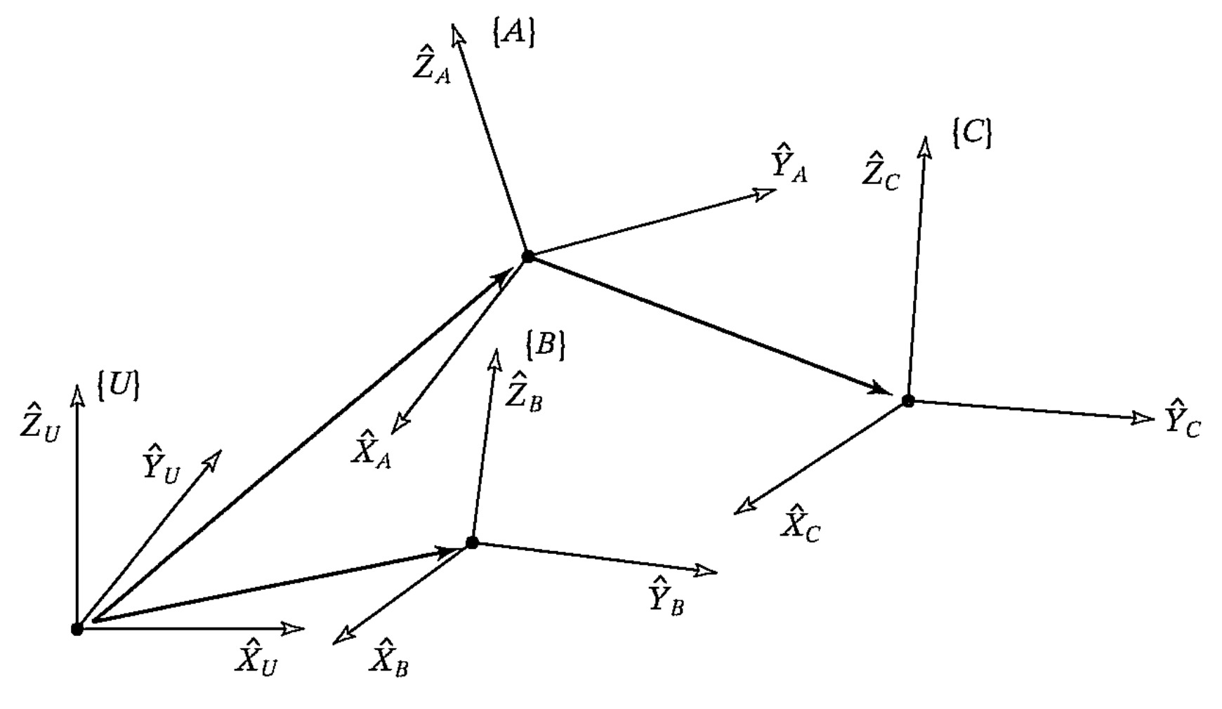
\[\{B\} = \{ {}^A_B R, \; {}^A\mathbf{P}_{B_{\text{ORG}}} \},\]where \({}^A\mathbf{P}_{B_{\text{ORG}}}\) is the vector locating the origin of ${B}$ expressed in ${A}$. Conceptually, a frame is a generalization of both a position (a frame whose rotation part is the identity) and an orientation (a frame whose origin coincides with the reference frame’s origin).
Geometrically, one may think of every frame as a triad of arrows (3 unit vectors) floating in space. A diagram of multiple frames typically shows arrows connecting one origin to another to indicate which frame is described relative to which.
Mappings
We turn now to the central computational problem: given the description of a quantity (a point, a vector) in one frame, compute its description in another frame. The geometric quantity does not change; only its description changes.
Translation
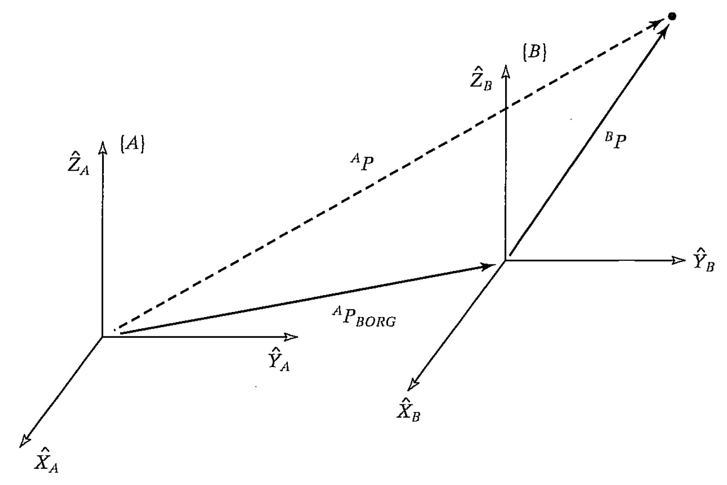
If $\{B\}$ differs from $\{A\}$ only by a translation—that is, $\{A\}$ and $\{B\}$ share the same orientation—then the mapping reduces to vector addition:
\[{}^A\mathbf{P} = {}^B\mathbf{P} + {}^A\mathbf{P}_{B_{\text{ORG}}}.\]This is only valid in the special case of equivalent orientations, where the components of ${}^B\mathbf{P}$ are already expressed along directions parallel to the axes of $\{A\}$.
Rotation
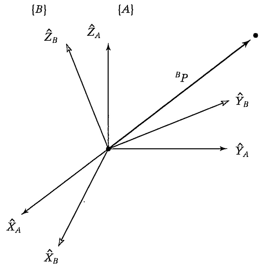
If instead $\{A\}$ and $\{B\}$ share an origin but differ in orientation, the mapping is implemented by a rotation matrix. Each component of ${}^A\mathbf{P}$ is the dot product of ${}^B\mathbf{P}$ with the corresponding axis of $\{A\}$ written in $\{B\}$:
\[\begin{aligned} {}^Ap_x &= {}^B\hat{X}_A \cdot {}^B\mathbf{P}, \\\\ {}^Ap_y &= {}^B\hat{Y}_A \cdot {}^B\mathbf{P}, \\\\ {}^Ap_z &= {}^B\hat{Z}_A \cdot {}^B\mathbf{P}. \end{aligned}\]Since the rows of ${}^A_B R$ are exactly ${}^B\hat{X}_A$, ${}^B\hat{Y}_A$, ${}^B\hat{Z}_A$, this collapses into the compact form
\[{}^A\mathbf{P} = {}^A_B R \; {}^B\mathbf{P}.\]A helpful mnemonic for the leading-script notation is to imagine the leading subscripts canceling the leading superscripts of the entity to their right.
General Frames
In the most general case $\{B\}$ is both rotated and translated relative to $\{A\}$. We first rotate ${}^B\mathbf{P}$ into an intermediate description with the same orientation as $\{A\}$, then add the translation that locates the origin of $\{B\}$ in $\{A\}$:
\[{}^A\mathbf{P} = {}^A_B R \; {}^B\mathbf{P} + {}^A\mathbf{P}_{B_{\text{ORG}}}.\]
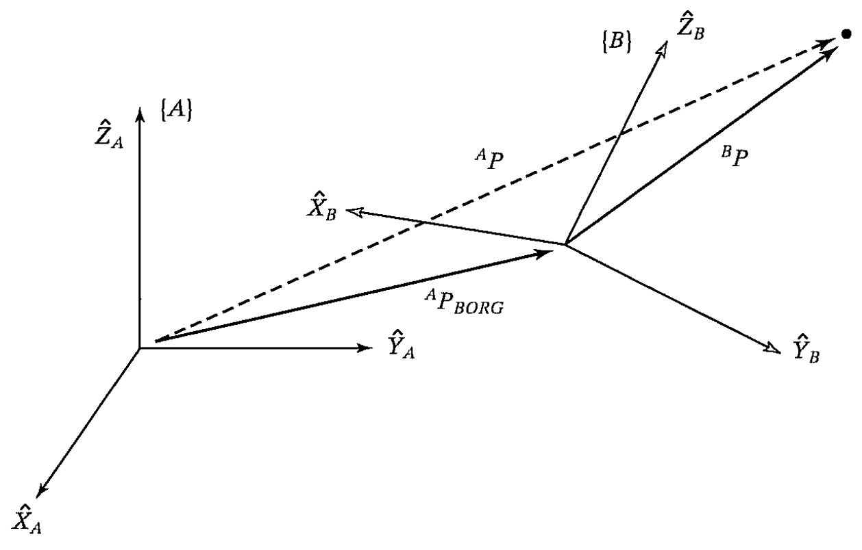
This is the fundamental rigid-body mapping. It is correct but a bit unsatisfying notationally; we would prefer to write a single matrix operator $T$ acting on a single vector to obtain the conceptual form
\[{}^A\mathbf{P} = {}^A_B T \; {}^B\mathbf{P}.\]This wish is granted by the homogeneous representation, introduced next.
Homogeneous Transformations and SE(3)
By appending a fourth coordinate “$1$” to every position vector and a fourth row “$[0\;0\;0\;1]$” to every transformation matrix, we obtain a single $4 \times 4$ block-matrix form that absorbs both rotation and translation:
\[\begin{bmatrix} {}^A\mathbf{P} \\ 1 \end{bmatrix} = \begin{bmatrix} {}^A_B R & {}^A\mathbf{P}_{B_{\text{ORG}}} \\ \mathbf{0} & 1 \end{bmatrix} \begin{bmatrix} {}^B\mathbf{P} \\ 1 \end{bmatrix}.\]The $4 \times 4$ matrix is the homogeneous transformation ${}^A_B T$:
\[{}^A_B T = \begin{bmatrix} {}^A_B R & {}^A\mathbf{P}_{B_{\text{ORG}}} \\ \mathbf{0} & 1 \end{bmatrix} \in \mathbb{R}^{4 \times 4}.\]Multiplying out reproduces both the rotation and the translation, with the trivial identity $1 = 1$.
The special Euclidean group of order 3 is the set of $4 \times 4$ homogeneous transformations of the form above, $$ SE(3) := \left\{ \begin{bmatrix} R & \mathbf{p} \\ \mathbf{0} & 1 \end{bmatrix} : R \in SO(3), \; \mathbf{p} \in \mathbb{R}^3 \right\}, $$ with matrix multiplication as the group operation. Elements of $SE(3)$ represent all rigid-body displacements (orientation plus position) in three-dimensional space.
Configuration Space of Rigid Bodies
Since a rigid body has fixed internal distances, we do not need to track every one of its material points separately. By stating its origin’s position $\mathbf{p} \in \mathbb{R}^3$ and its orientation $R \in SO(3)$ relative to a fixed inertial frame, we already fixes the position of every other point by rigidity. The pair $(R, \mathbf{p})$, equivalently the $4 \times 4$ matrix in $SE(3)$ we just defined, therefore contains all and only the information needed to say where the body is. This pair is called the body’s configuration, and the set of every configuration the body could conceivably occupy is its configuration space (C-Space).
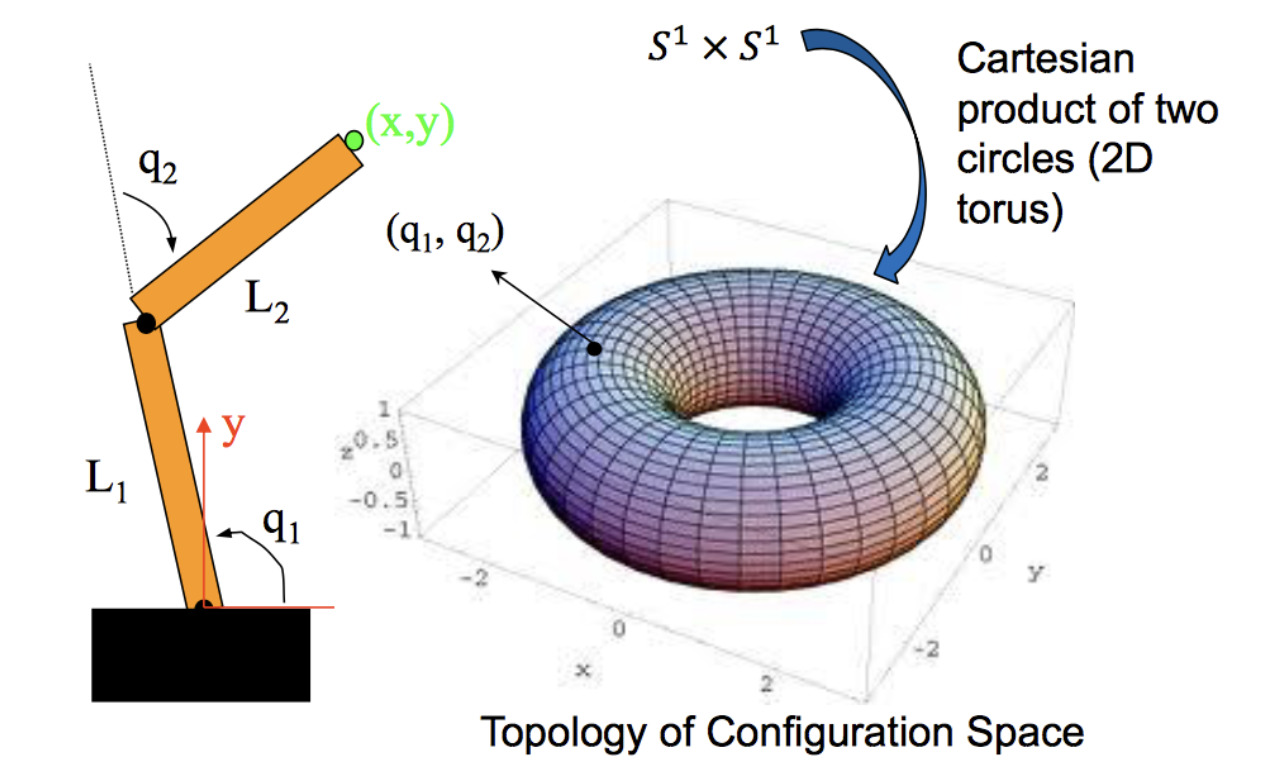
The observation that makes this entire post worth the trouble is that the configuration space is the very same object as the group $SE(3)$. The reason rests on two facts:
- Every configuration is reached from a chosen reference configuration by exactly one rigid-body displacement. Fix one configuration of the body as a reference (say, body frame coincident with the inertial frame). Any other configuration is obtained from the reference by a single rotation $R$ together with a single translation $\mathbf{p}$; conversely, applying any $(R, \mathbf{p}) \in SE(3)$ to the reference produces some configuration. Configurations and pairs $(R, \mathbf{p})$ stand in exact one-to-one correspondence.
- Rigid-body displacements are exactly the elements of $SE(3)$. Call a map $g : \mathbb{R}^3 \to \mathbb{R}^3$ a rigid-body transformation if it (i) preserves Euclidean distances between points and (ii) preserves the cross product of vectors. Property (i) alone would still admit mirror reflections; (ii) rules those out and selects the orientation-preserving isometries. One then proves that every such $g$ has the form $g(\mathbf{x}) = R\mathbf{x} + \mathbf{p}$ with $R \in SO(3)$ and $\mathbf{p} \in \mathbb{R}^3$—exactly the elements of $SE(3)$.
Combining these two facts: the configuration space of a rigid body in three dimensions is $SE(3)$.
- The body’s motion in time is a curve in $SE(3)$. The tangent vector to that curve at each instant packages the body’s angular and linear velocities into a single object called a twist—the central tool of the next post.
- Robot kinematics, dynamics, and motion planning all live on $SE(3)$. Forward kinematics maps joint angles to a point in $SE(3)$; inverse kinematics asks how to reach a target point in $SE(3)$; trajectory generation produces curves in $SE(3)$; feedback control regulates such curves. Phrasing each problem directly on the group, rather than on some chosen coordinate chart, makes the geometric structure visible and avoids the singularities of any particular parameterisation.
Interpretations
A single homogeneous transform admits multiple interpretations:
- Description of a frame. ${}^A_B T$ is the description of frame $\{B\}$ relative to $\{A\}$—its columns are the principal axes of $\{B\}$ in $\{A\}$ plus the origin offset.
- Mapping (change of description). ${}^A_B T$ maps ${}^B\mathbf{P} \mapsto {}^A\mathbf{P}$.
- Operator (active transformation). $T$ operates on a vector ${}^A\mathbf{P}_1$ to produce a new vector ${}^A\mathbf{P}_2 = T \, {}^A\mathbf{P}_1$ in the same frame.
These three views use identical mathematics; they differ only in interpretation, and the duality is the source of much of the elegance of rigid-body kinematics. The richest case is the equivalence between Use 1 (description) and Use 3 (operator): one and the same matrix $T(R, \mathbf{Q})$ may be read either as
- the operator that, applied to a point in $\{A\}$, rotates it by $R$ and translates it by $\mathbf{Q}$ (all within $\{A\}$) or
- the description of the frame $\{B\}$ obtained by rotating $\{A\}$ by $R$ and shifting its origin by $\mathbf{Q}$.
Both readings yield the same $4 \times 4$ matrix. For a concrete check, let $T = \mathrm{Trans}_z(10) \cdot \mathrm{Rot}_z(90^\circ)$. The operator reading sends a point $(1, 0, 0) \in \{A\}$ first to $(0, 1, 0)$ by the rotation and then to $(0, 1, 10)$ by the translation. The description reading interprets the same $T$ as ${}^A_B T$ of a frame $\{B\}$ whose origin sits at $(0, 0, 10)$ in $\{A\}$ and whose $\hat{X}_B$ axis points along $(0, 1, 0)$ in $\{A\}$—precisely the columns of $T$. Practically, this means the same matrix encodes both an active command (“move the gripper $10\,\mathrm{cm}$ along its $\hat{Z}$”) and a passive goal (“the new gripper pose lies $10\,\mathrm{cm}$ above the current one along $\hat{Z}$”).
Fixed-frame vs Body-frame Transformation
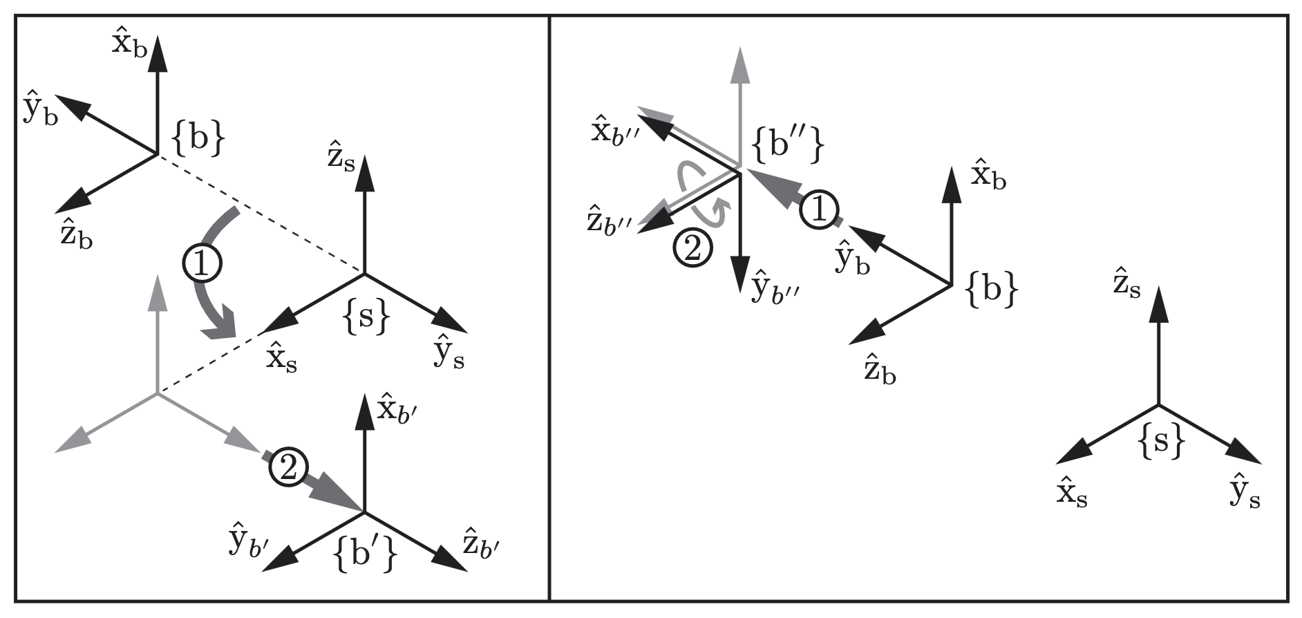
The operator use of a homogeneous transformation $T$ raises an immediate question: given a body at current pose $g$, should the additional transformation $T$ be applied as $T \cdot g$ or as $g \cdot T$? The two choices produce different results, each corresponding to a distinct physical reading: $T$ measured in the fixed (space) frame versus in the current (body) frame.
A single block-matrix calculation pins down the reason. Take $T$ to be a pure translation by $\mathbf{d} \in \mathbb{R}^3$ for clarity,
\[T = \begin{bmatrix} \mathbf{I} & \mathbf{d} \\ \mathbf{0}^\top & 1 \end{bmatrix}, \qquad g = \begin{bmatrix} \mathbf{R} & \mathbf{p} \\ \mathbf{0}^\top & 1 \end{bmatrix}.\]Pre-multiplying gives
\[T \cdot g = \begin{bmatrix} \mathbf{R} & \mathbf{p} + \mathbf{d} \\ \mathbf{0}^\top & 1 \end{bmatrix},\]while post-multiplying gives
\[g \cdot T = \begin{bmatrix} \mathbf{R} & \mathbf{p} + \mathbf{R}\mathbf{d} \\ \mathbf{0}^\top & 1 \end{bmatrix}.\]The only difference is whether $\mathbf{d}$ gets multiplied by $\mathbf{R}$ before being added. Since $\mathbf{R}$ converts body coordinates to space coordinates, $\mathbf{R}\mathbf{d}$ is “$\mathbf{d}$ read in body coordinates, then translated into space coordinates.” Pre-multiplication therefore treats $\mathbf{d}$ as already living in the fixed frame $\{A\}$, while post-multiplication treats $\mathbf{d}$ as living in the body frame $\{B\}$. The same conclusion holds for general $T$ with a rotation part.
| Composition | New translation | Interpretation of $T$ |
|---|---|---|
| $T \cdot g$ (pre-multiply) | $\mathbf{p} \to \mathbf{p} + \mathbf{d}$ | $T$ measured in fixed frame $\{A\}$ |
| $g \cdot T$ (post-multiply) | $\mathbf{p} \to \mathbf{p} + \mathbf{R}\mathbf{d}$ | $T$ measured in current body frame $\{B\}$ |
Compositions
Frames are often defined in chains. Suppose $\{C\}$ is known relative to $\{B\}$ via ${}^B_C T$, and $\{B\}$ is known relative to $\{A\}$ via ${}^A_B T$. Given a point known in $\{C\}$, we obtain its description in $\{A\}$ by first transforming through $\{B\}$:
\[{}^B\mathbf{P} = {}^B_C T \; {}^C\mathbf{P}, \qquad {}^A\mathbf{P} = {}^A_B T \; {}^B\mathbf{P}.\]Composing,
\[{}^A\mathbf{P} = {}^A_B T \; {}^B_C T \; {}^C\mathbf{P},\]so that the chained transform is simply the product
\[\boxed{\; {}^A_C T = {}^A_B T \; {}^B_C T \;}.\]In block form,
\[{}^A_C T = \begin{bmatrix} {}^A_B R \, {}^B_C R & {}^A_B R \, {}^B\mathbf{P}_{C_{\text{ORG}}} + {}^A\mathbf{P}_{B_{\text{ORG}}} \\\\ \mathbf{0} & 1 \end{bmatrix}.\]Inverses
Given ${}^A_B T$, the inverse ${}^B_A T = ({}^A_B T)^{-1}$ can be computed by exploiting the block structure rather than by general $4 \times 4$ matrix inversion. We seek \(({}^B_A R, {}^B\mathbf{P}_{A_{\text{ORG}}})\). Since rotation matrices invert by transposition, ${}^B_A R = {}^A_B R^T$. To obtain translation part, we change the description of $A$ into ${B}$:
\[\mathbf{0} = {}^B({}^A\mathbf{P}_{B_{\text{ORG}}}) = {}^B_A R {}^A\mathbf{P}_{B_{\text{ORG}}} + {}^B\mathbf{P}_{A_{\text{ORG}}}\]Then we have:
\[{}^B\mathbf{P}_{A_{\text{ORG}}} = -{}^A_B R^T \, {}^A\mathbf{P}_{B_{\text{ORG}}}.\]Assembling the block,
\[\boxed{\; {}^B_A T = \begin{bmatrix} {}^A_B R^T & -{}^A_B R^T \, {}^A\mathbf{P}_{B_{\text{ORG}}} \\ \mathbf{0} & 1 \end{bmatrix}. \;}\]Transform Equations and Loop Closure
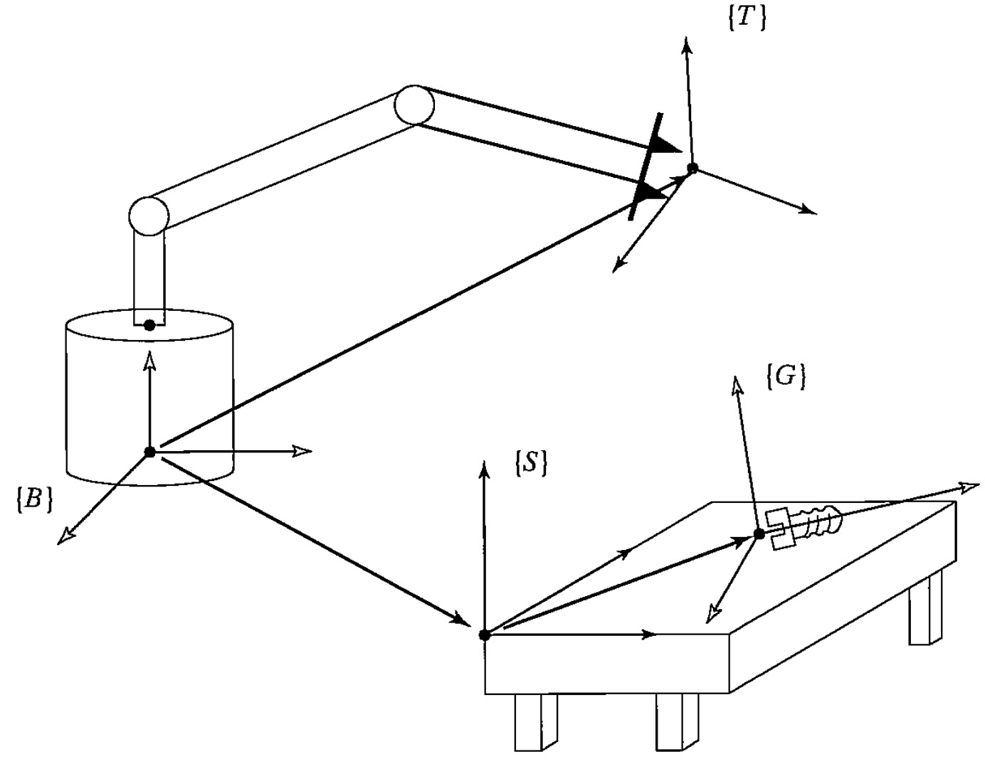
Many problems involve a set of frames connected in a loop, allowing a particular transform to be expressed in two different ways. Equating those expressions yields a transform equation that can be solved for an unknown.
For instance, suppose four frames $\{U\}, \{A\}, \{B\}, \{C\}, \{D\}$ are arranged such that
\[{}^U_D T = {}^U_A T \; {}^A_D T \qquad \text{and} \qquad {}^U_D T = {}^U_B T \; {}^B_C T \; {}^C_D T,\]then setting these two descriptions of ${}^U_D T$ equal,
\[{}^U_A T \; {}^A_D T = {}^U_B T \; {}^B_C T \; {}^C_D T,\]gives a single matrix equation. For example, for the following figure, we compute the bolt frame relative to the hand frame as:
\[{}^T_G T = {}^B_T T^{-1} \; {}^B_S T \; {}^S_G T.\]
Summary
We have built up, from scratch, the algebraic machinery used throughout robotics to describe and manipulate rigid-body configurations:
- A position is a $3 \times 1$ vector ${}^A\mathbf{P}$ tagged with its reference frame.
- An orientation is a $3 \times 3$ rotation matrix ${}^A_B R \in SO(3)$ whose columns are the principal axes of $\{B\}$ written in $\{A\}$.
- A frame \(\{B\} = \{ {}^A_B R, {}^A\mathbf{P}_{B_{\text{ORG}}} \}\) packages position and orientation, equivalently represented by a single $4 \times 4$ homogeneous transformation ${}^A_B T \in SE(3)$.
- A homogeneous transform admits three interpretations: description, mapping, operator.
- Transforms compose by matrix multiplication, ${}^A_C T = {}^A_B T \, {}^B_C T$, with index pattern-matching as a reliable shortcut.
- Transforms invert by the block formula \({}^B_A T = \begin{bmatrix} {}^A_B R^T & -{}^A_B R^T \, {}^A\mathbf{P}_{B_{\text{ORG}}} \\ \mathbf{0} & 1 \end{bmatrix}\).
- Transform equations arise whenever frames close into a loop and let us solve for any single unknown transform.
Every later topic in robot kinematics, dynamics, and control (forward kinematics, the manipulator Jacobian, screw theory, rigid-body dynamics) rests on the comfort with frames, rotations, and homogeneous transforms developed in this post.
Reference
[1] John J. Craig, Introduction to Robotics: Mechanics and Control, 3rd Edition, Pearson Prentice Hall, 2005. Chapter 2.
[2] Mark W. Spong, Seth Hutchinson, and M. Vidyasagar, Robot Dynamics and Control, 2nd Edition, January 2004. Chapter 2.
[3] Kevin M. Lynch and Frank C. Park, Modern Robotics: Mechanics, Planning, and Control, Cambridge University Press, 2017. Chapter 3.
[4] Richard M. Murray, Zexiang Li, and S. Shankar Sastry, A Mathematical Introduction to Robotic Manipulation, CRC Press, 1994. Chapter 2.
Leave a comment