
[Robotics] Rigid-Body Motion
Introduction
The configuration of a rigid body in $\mathbb{R}^3$ has six degrees of freedom, three for position and three for orientation. The set of all positions $\mathbb{R}^3$ is Euclidean, but the set of all orientations is not. This is the central conceptual obstacle that motivates the modern treatment of rigid-body motion. If we try to coordinatize orientations by Euler angles, roll-pitch-yaw, or any other three-parameter description, we inevitably encounter singularities (e.g., gimbal lock) and discontinuities. The reason for the obstruction is topological: the space of rotations $SO(3)$ is a curved three-dimensional manifold that admits no global, smooth chart from $\mathbb{R}^3$.
Problem: Gimbal Lock
A gimbal is a nested three-ring mechanism (originally used to stabilize compasses and gyroscopes) that rotates an inner body about three orthogonal axes. When the middle (pitch) ring reaches $\pm 90^\circ$, the outermost and innermost ring axes align in space, leaving only two independent rotation directions despite three physical rings.
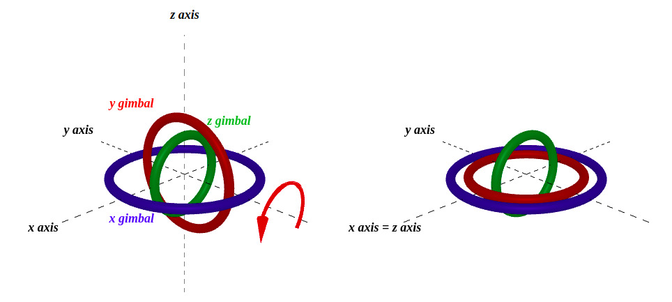
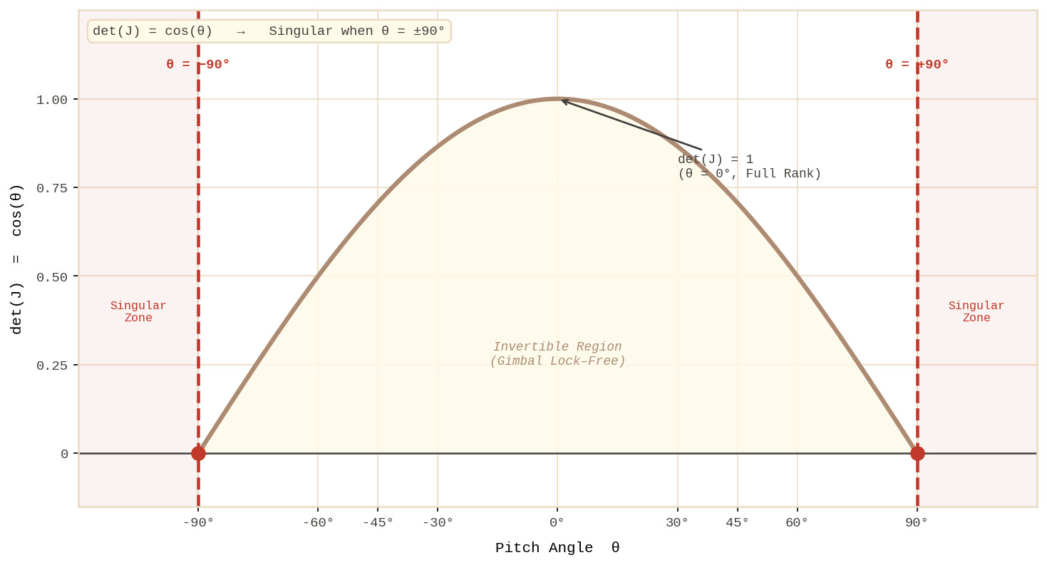
The mathematical mechanism behind gimbal lock can be made explicit. In the ZYX-Euler convention with yaw $\psi$, pitch $\theta$, and roll $\phi$, the body-frame angular velocity $\boldsymbol{\omega}_b$ is a linear function of the Euler-angle rates,
\[\boldsymbol{\omega}_b \;=\; J_b(\boldsymbol{\theta}) \begin{bmatrix} \dot{\phi} \\ \dot{\theta} \\ \dot{\psi} \end{bmatrix}, \qquad J_b(\boldsymbol{\theta}) \;=\; \begin{bmatrix} 1 & 0 & -\sin\theta \\ 0 & \cos\phi & \sin\phi\cos\theta \\ 0 & -\sin\phi & \cos\phi\cos\theta \end{bmatrix}.\]A direct expansion gives $\det J_b(\boldsymbol{\theta}) = \cos\theta$. At pitch $\theta = \pm \pi/2$ the Jacobian therefore becomes singular: the columns corresponding to $\dot{\phi}$ and $\dot{\psi}$ collapse onto the same direction in $\boldsymbol{\omega}_b$-space, so one independent rotational rate is irrecoverably lost. Gimbal lock is not a flaw of any specific convention; it is forced by the topological mismatch between $\mathbb{R}^3$ and $SO(3)$.
The singularity also surfaces at the code level. A standard quaternion-to-ZYX-Euler conversion is
1
2
3
4
5
6
7
8
9
10
11
12

import numpy as np

def quaternion_to_euler_zyx(w, x, y, z):
    # Roll (φ, X-axis rotation)
    roll = np.arctan2(2*(w*x + y*z), 1 - 2*(x*x + y*y))
    # Pitch (θ, Y-axis rotation)
    sin_pitch = 2*(w*y - z*x)
    sin_pitch = np.clip(sin_pitch, -1.0, 1.0)
    pitch = np.arcsin(sin_pitch)
    # Yaw (ψ, Z-axis rotation)
    yaw = np.arctan2(2*(w*z + x*y), 1 - 2*(y*y + z*z))
    return roll, pitch, yaw
Near pitch $\theta = \pm \pi/2$, the arguments of both the roll and yaw arctan2 calls approach zero. Since atan2(0, 0) is undefined, tiny floating-point errors there are amplified into wild swings in the roll and yaw outputs.
Topology of $SO(3)$
Gimbal lock is not a defect of a particular Euler-angle convention. The explanation lies in the topology of $SO(3)$.
Shape of $SO(3)$
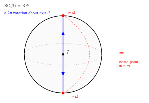
Every rotation can be represented by an axis-angle pair $\theta\,\hat{\boldsymbol{\omega}}$, with $\theta\in[-\pi,\pi]$. These vectors fill a solid ball $B^3$ of radius $\pi$. The representation is unique except on the boundary: a rotation by $\pi$ about $\hat{\boldsymbol\omega}$ is identical to a rotation by $\pi$ about $-\hat{\boldsymbol\omega}$. Consequently, antipodal boundary points must be identified. The resulting quotient space is real projective 3-space $\mathbb{RP}^3$, and $SO(3)$ has exactly this shape (called homeomorphic; see the proof).
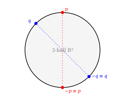
The antipodal identification introduces a non-contractible loop. Starting at the center of $B^3$ (the identity rotation $\mathbf{I}$), travel to a boundary point $\pi\hat{\boldsymbol\omega}$, continue from the antipodal point $-\pi\hat{\boldsymbol\omega}$, and return to the center. Because the boundary points are identified, this path closes into a loop in $SO(3)$ and cannot be shrunk to a point while remaining in the space.
As a rotation, the loop represents a single $2\pi$ turn about $\hat{\boldsymbol\omega}$. Traversing it twice yields a $4\pi$ rotation, which is then contractible. This is the topological origin of the Dirac belt trick.
The non-contractible loop above already reveals that $SO(3)$ has nontrivial topology. A more geometric manifestation of the same obstruction appears on the sphere $S^2$ through the Hairy Ball Theorem: there is no nonvanishing continuous tangent vector field on odd-dimensional spheres. Informally, one cannot comb the hair on a sphere flat without creating a cowlick, and no latitude–longitude chart can remain regular everywhere.
The non-contractible loop above shows that $SO(3)$ has nontrivial topology. To see how this topology obstructs Euler-angle coordinates, it is useful to project $SO(3)$ onto a simpler space where the obstruction is easier to visualize: the sphere $S^2$. Fix a body-fixed $x$-axis \(\hat{\mathbf{e}}_1\). Every rotation $R\in SO(3)$ sends it to a unit vector \(R \hat{\mathbf{e}}_1 \in S^2\), defining the projection
\[p:SO(3)\rightarrow S^2, \qquad R\mapsto R \hat{\mathbf{e}}_1.\]Geometrically, this projection forgets rotations about the axis \(R\hat{\mathbf{e}}_1\) and remembers only where the axis points. The remaining degree of freedom is a rotation about \(R\hat{\mathbf{e}}_1\), so above each point of $S^2$ sits a circle $S^1$. In this sense, $SO(3)$ can be viewed as a circle bundle over the sphere.
For ZYX Euler angles $(\psi,\theta,\phi)$, the first two angles $(\psi,\theta)$ determine the pointing direction \(R\hat{\mathbf{e}}_1\), and the third angle $\phi$ specifies the residual rotation about that direction. Thus $(\psi,\theta)$ define a coordinate chart on $S^2$: a smooth assignment of two coordinates to each pointing direction, analogous to longitude and latitude on the Earth. If this chart were globally regular, varying the coordinate $\psi$ would produce a nonzero tangent direction at every point of the sphere. In other words, the coordinate vector field $\partial_\psi$ would be a continuous tangent vector field that never vanishes.
The Hairy Ball Theorem states that no such field exists on $S^2$. Every continuous tangent vector field on the sphere must vanish somewhere. Therefore the Euler-angle chart must become singular at some point. For ZYX Euler angles, the singularities occur at
\[\theta=\pm\frac{\pi}{2},\]where the body axis \(\hat{\mathbf{e}}_1\) points straight up or down. At these poles, changing the yaw angle $\psi$ no longer changes the pointing direction \(R\hat{\mathbf{e}}_1\); the vector field $\partial_\psi$ vanishes and the chart degenerates.

Lie Group Theory for Rigid Body Motions
For this reason, modern robotics works directly on $SO(3)$ as a matrix Lie group rather than through a global coordinate chart. Local coordinates are supplied by the Lie algebra $\mathfrak{so}(3)$ through the exponential map. This viewpoint extends naturally to $SE(3)$, provides a unified language for rotations, angular velocities, twists, and rigid-body motions, and underlies modern formulations such as the product-of-exponentials representation, geometric Jacobians, and Newton–Euler dynamics.
Preliminary: Lie Group Theory for Rigid Body Motions
The covering-map argument above ruled out a smooth bijection $\mathbb{R}^3 \to SO(3)$, but it does not rule out useful coordinates altogether. The right framework is Lie theory: a body of structure theory that simultaneously handles a smooth manifold and a group operation, and provides three universal tools, an algebra, an exponential, and (later) an adjoint, which specialize to give every concrete calculation we need for $SO(3)$ and $SE(3)$. We collect the abstract definitions here so the sections that follow can be read as instantiations of the same pattern.
Group Theory
A group abstracts the algebraic structure of operations that can be composed and undone. Rotations of a rigid body, displacements of a robot, permutations of a list, and the integers under addition are all groups; the four axioms below capture exactly what such “compose-and-undo” calculus requires.
A group $(G, \cdot)$ is a set $G$ equipped with a binary operation $\cdot : G \times G \to G$, written $(a, b) \mapsto a \cdot b$, satisfying the following four axioms:
- Closure. $a \cdot b \in G$ for all $a, b \in G$.
- Associativity. $(a \cdot b) \cdot c = a \cdot (b \cdot c)$ for all $a, b, c \in G$.
- Identity. There exists $e \in G$ such that $e \cdot a = a \cdot e = a$ for every $a \in G$.
- Inverse. For each $a \in G$ there exists $a^{-1} \in G$ such that $a \cdot a^{-1} = a^{-1} \cdot a = e$.
Many groups of interest in robotics arise inside a larger ambient group. $SO(3)$, for instance, sits inside the general linear group $GL(3, \mathbb{R})$ of invertible $3 \times 3$ real matrices, both under matrix multiplication. Such an inherited group structure is called a subgroup.
A subgroup $H$ of a group $(G, \cdot)$ is a subset $H \subseteq G$ that is itself a group under the restriction of the group operation. Concretely, $H \subseteq G$ is a subgroup if and only if it is non-empty, closed under the group operation ($h_1, h_2 \in H \Rightarrow h_1 \cdot h_2 \in H$), and closed under inverses ($h \in H \Rightarrow h^{-1} \in H$); the identity $e \in H$ then follows automatically.
Some spaces of interest carry both vector-space structure (closed under addition and scalar multiplication) and a multiplicative product on top. The $n \times n$ real matrices are the canonical example: as a set they form a vector space, but they also admit matrix multiplication, which combines two matrices into another. Such a structure, a vector space carrying a compatible multiplication, is called an algebra.
An algebra over $\mathbb{R}$ is a real vector space $V$ equipped with an additional binary operation $V \times V \to V$ (called the product of the algebra) that is bilinear: it distributes over vector addition and commutes with scalar multiplication in each argument. The product is not required to be associative or commutative.
For a thorough introduction to group theory and its application to rigid-body motion, see Gallo [7].
Manifolds and Tangent Spaces
A Lie group is a group that is also a smooth (inifinitely differentiable) manifold, and the algebra is its tangent space at the identity. We recall both notions briefly, since they appear in every subsequent definition.
A $d$-dimensional manifold $\mathcal{M}$ is a topological space in which every point has a neighborhood that is homeomorphic to an open subset of $\mathbb{R}^d$. Informally, $\mathcal{M}$ is a $d$-dimensional curved object that looks flat at any sufficiently small scale: the surface of a sphere is a 2-manifold sitting in $\mathbb{R}^3$, and the rotation group $SO(3)$ is a 3-manifold sitting in $\mathbb{R}^9$.
On any smooth manifold, each point carries a linearization called tangent space: the vector space of all velocities through that point.
The tangent space $T_x \mathcal{M}$ at a point $x \in \mathcal{M}$ is the $d$-dimensional real vector space of velocities $\dot{\gamma}(0)$ of smooth curves $\gamma : (-\varepsilon, \varepsilon) \to \mathcal{M}$ with $\gamma(0) = x$. Geometrically, $T_x \mathcal{M}$ is the flat hyperplane that best approximates $\mathcal{M}$ at $x$.
Being flat, the tangent space is amenable to ordinary linear algebra. The bridge between the manifold and its tangent space at a chosen base point is the exponential map, a general construction whose form depends on what additional structure the manifold carries.
On a smooth manifold $\mathcal{M}$ equipped with additional structure that picks out, for each tangent vector $v \in T_p \mathcal{M}$, a canonical smooth curve $\gamma_v : (-\varepsilon, \varepsilon) \to \mathcal{M}$ with $\gamma_v(0) = p$ and $\dot{\gamma}_v(0) = v$, the exponential map at $p$ is $$\exp_p \,:\, U \subseteq T_p \mathcal{M} \,\to\, \mathcal{M}, \qquad v \,\mapsto\, \gamma_v(1).$$ The logarithm map $\log_p$ is the local inverse on a neighborhood of $p$ where $\exp_p$ is a diffeomorphism.
The “canonical curve $\gamma_v$” comes from whatever additional structure the manifold carries, and three instantiations cover essentially all the cases used in robotics:
- Riemannian manifold. $\gamma_v$ is the unique geodesic with $\gamma_v(0) = p$ and $\dot{\gamma}_v(0) = v$, so $\exp_p$ is the standard Riemannian exponential.
- Lie group $G$. At the canonical base point $p = \mathbf{I}$, $\gamma_X$ is the unique smooth one-parameter subgroup ($\gamma_X(s + t) = \gamma_X(s)\gamma_X(t)$) with $\dot{\gamma}_X(0) = X$. This gives $\exp : \mathfrak{g} \to G$ with $\mathfrak{g} := T_{\mathbf{I}} G$.
- Matrix Lie group $G \subset GL(n, \mathbb{R})$. The Lie group case specializes to the absolutely convergent matrix series $$\exp(X) \;=\; \sum_{k=0}^\infty \frac{X^k}{k!}, \qquad \log(\mathbf{I} + M) \;=\; \sum_{k=1}^\infty (-1)^{k-1} \frac{M^k}{k}.$$
For Lie groups with a bi-invariant Riemannian metric (which includes $SO(3)$ but not $SE(3)$), instantiations 1 and 2 agree at the identity. Throughout the rest of the post we use case 3, the matrix specialization.
Matrix Lie Groups and Lie Algebras
The most general matrix group is the general linear group \(GL(n, \mathbb{R}) := \{A \in \mathbb{R}^{n \times n} : \det(A) \neq 0\}\), the set of invertible $n \times n$ real matrices with matrix multiplication as the group operation. Every matrix Lie group of interest in robotics sits inside $GL(n, \mathbb{R})$ as a subgroup that is also a smooth submanifold; the orthogonal group $O(n)$, the special orthogonal group $SO(n)$, and the special Euclidean group $SE(n)$ are all of this form.
A matrix Lie group $G$ is a subgroup of $GL(n, \mathbb{R})$ that is also a smooth submanifold of $\mathbb{R}^{n \times n}$, with the group operation and inversion being smooth. Its Lie algebra $\mathfrak{g}$ is the tangent space to $G$ at the identity matrix $\mathbf{I}$, $$\mathfrak{g} \;:=\; T_{\mathbf{I}} G \;=\; \{ \dot{g}(0) \,:\, g(t) \in G,\, g(0) = \mathbf{I} \} \;\subset\; \mathbb{R}^{n \times n},$$ a vector subspace of $n \times n$ matrices. It inherits a Lie bracket from the matrix commutator $[X, Y] := XY - YX$, which lands back in $\mathfrak{g}$ and measures the failure of two infinitesimal motions to commute.
For $SO(3)$ and $SE(3)$ the log map admits a closed form (Section on $\mathfrak{so}(3)$ below); together $(\exp, \log)$ are the round-trip between the group and its algebra used by every modern on-manifold optimization, control, and state-estimation algorithm. In short, the recipe for rigid-body motion is then the same one in two places: identify the group ($SO(3)$ or $SE(3)$), compute its tangent space at the identity to find the algebra ($\mathfrak{so}(3)$ or $\mathfrak{se}(3)$), and use the matrix exponential to move between them. In this post we will instantiate this process: angular velocity $\leftrightarrow \mathfrak{so}(3) \leftrightarrow \exp \leftrightarrow$ rotation, and twist $\leftrightarrow \mathfrak{se}(3) \leftrightarrow \exp \leftrightarrow$ rigid motion.
Rigid Body Motion
Before going further, we need precise definitions of two basic notions: a rigid body, and a rigid-body transformation.
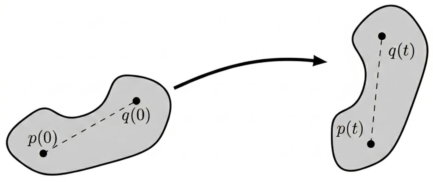
An object $\mathcal{O} \subset \mathbb{R}^3$ is a rigid body if the distance between any two of its particles is invariant under any motion of the object. Equivalently, if $\mathbf{p}(t), \mathbf{q}(t) \in \mathbb{R}^3$ denote the positions of two particles at time $t$, then $$ \Vert \mathbf{p}(t) - \mathbf{q}(t) \Vert \;=\; \Vert \mathbf{p}(0) - \mathbf{q}(0) \Vert \qquad \text{for all } t \geq 0. $$
The definition above describes the body itself; we also need the corresponding class of maps that move it through space.
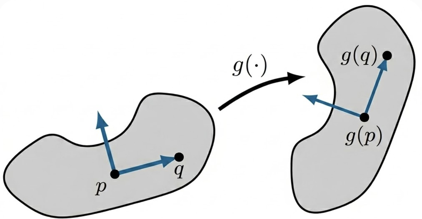
A mapping $T : \mathbb{R}^3 \to \mathbb{R}^3$ is a rigid body transformation if it satisfies
- Length preservation. $\Vert T(\mathbf{p}) - T(\mathbf{q}) \Vert = \Vert \mathbf{p} - \mathbf{q} \Vert$ for all $\mathbf{p}, \mathbf{q} \in \mathbb{R}^3$.
- Cross-product preservation. $T_*(\mathbf{v} \times \mathbf{w}) = T_*(\mathbf{v}) \times T_*(\mathbf{w})$ for all $\mathbf{v}, \mathbf{w} \in \mathbb{R}^3$, where $T_*$ is the induced map on vectors of rigid body $T_*(\mathbf{v} = \mathbf{q} - \mathbf{p}) := T(\mathbf{q}) - T(\mathbf{p})$ for any $\mathbf{p}, \mathbf{q} \in \mathbb{R}^3$.
A rigid-body transformation is, in particular, an isometry of $\mathbb{R}^3$: a map that preserves distances between points, or equivalently, distances from any fixed point together with the angles at that point. Length preservation alone, however, admits both rotations and reflections. Condition 2 rules out reflections by continuity: physical motion is continuous, so each tiny step shifts the axes only slightly and never flips them, keeping a right-handed frame right-handed. Together the two conditions characterize the orientation-preserving isometries of $\mathbb{R}^3$: the rotations $SO(3)$ (origin-fixing) and the rigid motions $SE(3)$ (with translation), developed below.
Space and Body Frames
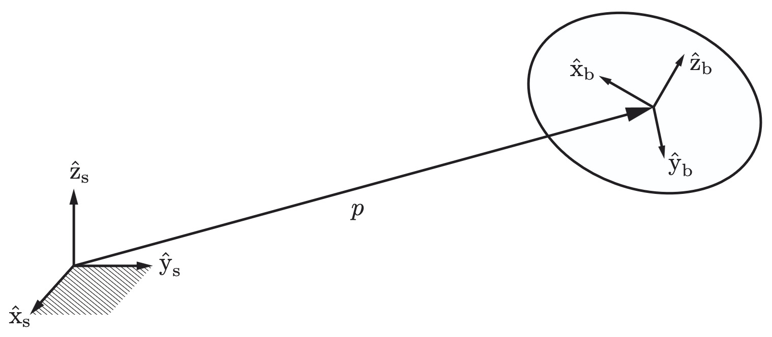
For the description of rigid body motion we always assume one stationary space frame \(\{s\}\), attached to some fixed location such as a corner of a room. To each moving rigid body we attach a body frame \(\{b\}\), defined as the stationary frame that is coincident with the body-attached frame at any given instant.
Rotations: $SO(3)$ and $\mathfrak{so}(3)$
Rotation Matrices and $SO(3)$
The rotation group $SO(3)$ is the simplest non-trivial matrix Lie group used in robotics: a smooth three-dimensional subset of $GL(3, \mathbb{R})$ whose group operation is matrix multiplication. We unpack this concretely. Recall that the three columns of a rotation matrix \(\mathbf{R}_{sb}\) correspond to the body-frame unit axes \(\hat{\mathbf{x}}_b, \hat{\mathbf{y}}_b, \hat{\mathbf{z}}_b\) expressed in the space frame \(\{s\}\):
\[\mathbf{R}_{sb} = \begin{bmatrix} \hat{\mathbf{x}}_b & \hat{\mathbf{y}}_b & \hat{\mathbf{z}}_b \end{bmatrix} \in \mathbb{R}^{3\times 3}.\]The following conditions must therefore be satisfied:
- Unit norm. Each column is a unit vector: $\hat{\mathbf{x}}_b \cdot \hat{\mathbf{x}}_b = \hat{\mathbf{y}}_b \cdot \hat{\mathbf{y}}_b = \hat{\mathbf{z}}_b \cdot \hat{\mathbf{z}}_b = 1$.
- Mutual orthogonality. Distinct columns are orthogonal: $\hat{\mathbf{x}}_b \cdot \hat{\mathbf{y}}_b = \hat{\mathbf{y}}_b \cdot \hat{\mathbf{z}}_b = \hat{\mathbf{z}}_b \cdot \hat{\mathbf{x}}_b = 0$.
- Right-handedness. The triple forms a right-handed frame: $\hat{\mathbf{x}}_b \times \hat{\mathbf{y}}_b = \hat{\mathbf{z}}_b$.
The first two give six explicit constraints, summarized compactly as \(\mathbf{R}_{sb}^{\top} \mathbf{R}_{sb} = \mathbf{I}\). The third translates into a determinant condition through the scalar triple product identity, which expresses the determinant of a $3 \times 3$ matrix with columns $\mathbf{a}, \mathbf{b}, \mathbf{c}$ as
\[\det [\,\mathbf{a} \mid \mathbf{b} \mid \mathbf{c}\,] \;=\; \mathbf{a} \cdot (\mathbf{b} \times \mathbf{c}) \;=\; \mathbf{b} \cdot (\mathbf{c} \times \mathbf{a}) \;=\; \mathbf{c} \cdot (\mathbf{a} \times \mathbf{b}).\]Applied to $\mathbf{R}_{sb}$ and combined with the cyclic permutation $\hat{\mathbf{y}}_b \times \hat{\mathbf{z}}_b = \hat{\mathbf{x}}_b$ of the right-hand rule $\hat{\mathbf{x}}_b \times \hat{\mathbf{y}}_b = \hat{\mathbf{z}}_b$,
\[\det \mathbf{R}_{sb} \;=\; \hat{\mathbf{x}}_b \cdot (\hat{\mathbf{y}}_b \times \hat{\mathbf{z}}_b) \;=\; \hat{\mathbf{x}}_b \cdot \hat{\mathbf{x}}_b \;=\; 1.\]A left-handed frame would instead give \(\hat{\mathbf{y}}_b \times \hat{\mathbf{z}}_b = -\hat{\mathbf{x}}_b\) and hence \(\det \mathbf{R}_{sb} = -1\), so right-handedness is exactly the condition \(\det \mathbf{R}_{sb} = +1\).
The special orthogonal group $SO(3)$, also known as the group of rotation matrices, is the set of all $3 \times 3$ real matrices $R$ that satisfy $$ SO(3) := \left\{ \mathbf{R} \in \mathbb{R}^{3\times 3} : \mathbf{R}^{\top}\mathbf{R} = \mathbf{I}, \; \det \mathbf{R} = +1 \right\}. $$
$SO(3)$ as a group
Specializing the group axioms to $SO(3)$ with matrix multiplication as the group operation:
- Closure. If $\mathbf{R}_1, \mathbf{R}_2 \in SO(3)$, then $(\mathbf{R}_1\mathbf{R}_2)(\mathbf{R}_1\mathbf{R}_2)^{\top} = \mathbf{R}_1\mathbf{R}_2\mathbf{R}_2^{\top}\mathbf{R}_1^{\top} = \mathbf{I}$, and $\det(\mathbf{R}_1\mathbf{R}_2) = (+1)(+1) = +1$.
- Identity. $\mathbf{I} \in SO(3)$.
- Inverse. $\mathbf{R}^{-1} = \mathbf{R}^{\top} \in SO(3)$.
- Associativity. Inherited from matrix multiplication.
Rotations preserve geometry. A rigid-body transformation must preserve distances and orientation (handedness). For the cross product, one has the useful algebraic identity
\[\mathbf{R}(\mathbf{v} \times \mathbf{w}) = (\mathbf{R}\mathbf{v}) \times (\mathbf{R}\mathbf{w}), \qquad \mathbf{R} \in SO(3).\]Distance preservation is direct:
\[\Vert \mathbf{R}\mathbf{q} - \mathbf{R}\mathbf{p} \Vert^2 = (\mathbf{q}-\mathbf{p})^{\top}\mathbf{R}^{\top}\mathbf{R}(\mathbf{q}-\mathbf{p}) = \Vert\mathbf{q}-\mathbf{p}\Vert^2.\]Thus every $\mathbf{R} \in SO(3)$ is a rigid body transformation, and orientation is preserved because $\det \mathbf{R} = +1$ excludes reflections.
Angular Velocities and $\mathfrak{so}(3)$
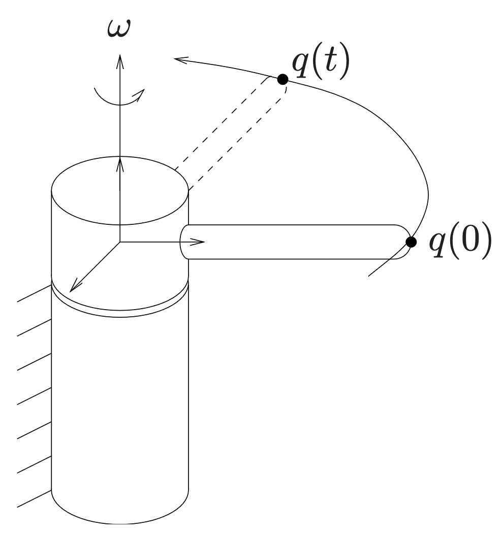
Picture a rigid body rotating relative to the space frame ${s}$, with its instantaneous orientation captured by $\mathbf{R}(t) \in SO(3)$. Take $\mathbf{q}_b \in \mathbb{R}^3$ that is fixed in \(\{b\}\), so $\mathbf{q}_b$ is constant in time. Its spatial-frame position is $\mathbf{q}(t) = \mathbf{R}(t)\, \mathbf{q}_b$, and its velocity in ${s}$ is
\[\dot{\mathbf{q}}(t) \;=\; \dot{\mathbf{R}}(t)\, \mathbf{q}_b \;=\; \dot{\mathbf{R}}(t)\, \mathbf{R}(t)^\top\, \mathbf{q}(t).\]The map taking each current spatial position $\mathbf{q}$ to its current velocity $\dot{\mathbf{q}}$ is therefore the matrix $\dot{\mathbf{R}}\, \mathbf{R}^\top$, regardless of which body-fixed point we picked. Differentiating the orthogonality constraint $\mathbf{R}(t)\, \mathbf{R}(t)^\top = \mathbf{I}$,
\[\dot{\mathbf{R}}\, \mathbf{R}^\top + \mathbf{R}\, \dot{\mathbf{R}}^\top \;=\; \mathbf{0} \quad\Longrightarrow\quad \dot{\mathbf{R}}\, \mathbf{R}^\top \;=\; -\bigl(\dot{\mathbf{R}}\, \mathbf{R}^\top\bigr)^\top,\]shows that $\dot{\mathbf{R}}\, \mathbf{R}^\top$ is skew-symmetric. Any $3 \times 3$ skew matrix acts on vectors as a cross product $\boldsymbol{\omega} \times (\cdot)$ for a unique $\boldsymbol{\omega} \in \mathbb{R}^3$, so writing $\dot{\mathbf{R}}\, \mathbf{R}^\top = [\boldsymbol{\omega}]$ turns the velocity formula into the familiar
\[\dot{\mathbf{q}}(t) \;=\; \boldsymbol{\omega}(t) \times \mathbf{q}(t).\]
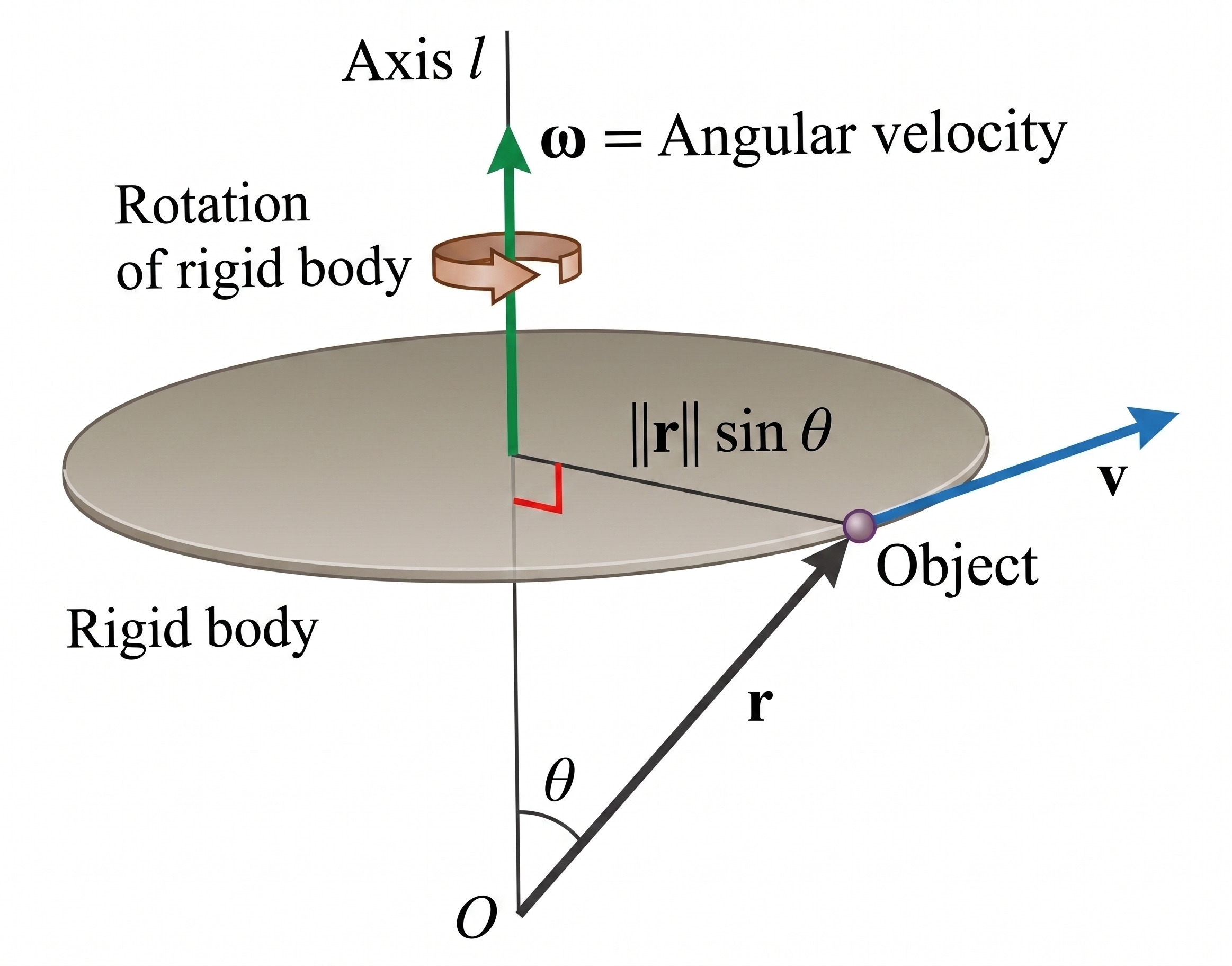
In coordinates, the skew matrix associated with $\boldsymbol{\omega} = (\omega_1, \omega_2, \omega_3)$ acts on a vector $\mathbf{q} = (q_1, q_2, q_3)$ as
\[[\boldsymbol{\omega}]\, \mathbf{q} \;=\; \begin{bmatrix} 0 & -\omega_3 & \omega_2 \\ \omega_3 & 0 & -\omega_1 \\ -\omega_2 & \omega_1 & 0 \end{bmatrix} \begin{bmatrix} q_1 \\ q_2 \\ q_3 \end{bmatrix} \;=\; \begin{bmatrix} \omega_2 q_3 - \omega_3 q_2 \\ \omega_3 q_1 - \omega_1 q_3 \\ \omega_1 q_2 - \omega_2 q_1 \end{bmatrix} \;=\; \boldsymbol{\omega} \times \mathbf{q},\]The vector $\boldsymbol{\omega}(t) \in \mathbb{R}^3$ is the angular velocity of the body: its direction is the (instantaneous, right-handed) axis of rotation, and its magnitude is the rate of rotation. The matrix $\dot{\mathbf{R}}\, \mathbf{R}^\top$ lives in the space of $3 \times 3$ skew-symmetric matrices, which we will identify as the Lie algebra $\mathfrak{so}(3)$ of $SO(3)$.
Spatial and Body angular velocity
The differentiation argument actually produces two skew matrices, depending on which side of $\mathbf{R}$ we put the derivative on:
\[[\boldsymbol{\omega}_s] := \dot{\mathbf{R}}\mathbf{R}^\top \,\in\, \mathfrak{so}(3), \qquad [\boldsymbol{\omega}_b] := \mathbf{R}^\top\dot{\mathbf{R}} \,\in\, \mathfrak{so}(3).\]These encode the same physical rotation rate expressed in two different frames: $\boldsymbol{\omega}_s$ is the spatial angular velocity (expressed in the fixed frame ${s}$), and $\boldsymbol{\omega}_b$ is the body angular velocity (expressed in the rotating frame ${b}$). To relate the two we need the following identity, which lets a rotation pass through the hat operator.
For any $\mathbf{R} \in SO(3)$ and $\boldsymbol{\omega} \in \mathbb{R}^3$, $$\mathbf{R}\, [\boldsymbol{\omega}]\, \mathbf{R}^\top \;=\; [\mathbf{R}\, \boldsymbol{\omega}].$$
$\color{#bf1100}{\mathbf{Proof.}}$
Apply both sides to an arbitrary test vector $\mathbf{v} \in \mathbb{R}^3$ and use $[\boldsymbol{\omega}]\mathbf{u} = \boldsymbol{\omega} \times \mathbf{u}$ together with the cross-product preservation property of rotations, $\mathbf{R}(\mathbf{a} \times \mathbf{b}) = (\mathbf{R}\mathbf{a}) \times (\mathbf{R}\mathbf{b})$ for $\mathbf{R} \in SO(3)$:
\[\mathbf{R}\, [\boldsymbol{\omega}]\, \mathbf{R}^\top\, \mathbf{v} \;=\; \mathbf{R}\bigl(\boldsymbol{\omega} \times \mathbf{R}^\top \mathbf{v}\bigr) \;=\; (\mathbf{R}\, \boldsymbol{\omega}) \times (\mathbf{R}\mathbf{R}^\top \mathbf{v}) \;=\; (\mathbf{R}\, \boldsymbol{\omega}) \times \mathbf{v} \;=\; [\mathbf{R}\, \boldsymbol{\omega}]\, \mathbf{v}.\]Since the equality holds for every $\mathbf{v}$, $\mathbf{R}[\boldsymbol{\omega}]\mathbf{R}^\top = [\mathbf{R}\boldsymbol{\omega}]$. $\blacksquare$
Applying this proposition with $\boldsymbol{\omega} = \boldsymbol{\omega}_b$, and using $\mathbf{R}\mathbf{R}^\top = \mathbf{I}$ to insert an identity in the middle,
\[[\boldsymbol{\omega}_s] \;=\; \dot{\mathbf{R}}\, \mathbf{R}^\top \;=\; \mathbf{R}\, (\mathbf{R}^\top \dot{\mathbf{R}})\, \mathbf{R}^\top \;=\; \mathbf{R}\, [\boldsymbol{\omega}_b]\, \mathbf{R}^\top \;=\; [\mathbf{R}\, \boldsymbol{\omega}_b].\]Therefore, we obtain $\boldsymbol{\omega}_s = \mathbf{R}\, \boldsymbol{\omega}_b$.
Frame-independence. The spatial angular velocity \(\boldsymbol{\omega}_s\) does not depend on the choice of body frame \(\{b\}\), and the body angular velocity \(\boldsymbol{\omega}_b\) does not depend on the choice of spatial frame \(\{s\}\). Replacing \(\{b\}\) with another body-fixed frame \(\{b'\}\) amounts to right-multiplying \(\mathbf{R}_{sb}\) by a constant rotation \(\mathbf{R}_{bb'}\) (constant since both frames are rigidly attached to the body):
\[\dot{\mathbf{R}}_{sb'}\, \mathbf{R}_{sb'}^\top \;=\; (\dot{\mathbf{R}}_{sb}\, \mathbf{R}_{bb'})\, (\mathbf{R}_{sb}\, \mathbf{R}_{bb'})^\top \;=\; \dot{\mathbf{R}}_{sb}\, \mathbf{R}_{bb'}\, \mathbf{R}_{bb'}^\top\, \mathbf{R}_{sb}^\top \;=\; \dot{\mathbf{R}}_{sb}\, \mathbf{R}_{sb}^\top \;=\; [\boldsymbol{\omega}_s].\]A symmetric calculation shows \([\boldsymbol{\omega}_b] = \mathbf{R}_{sb}^\top\, \dot{\mathbf{R}}_{sb}\) is unchanged under any constant change of the spatial frame.
Lie algebra $\mathfrak{so}(3)$
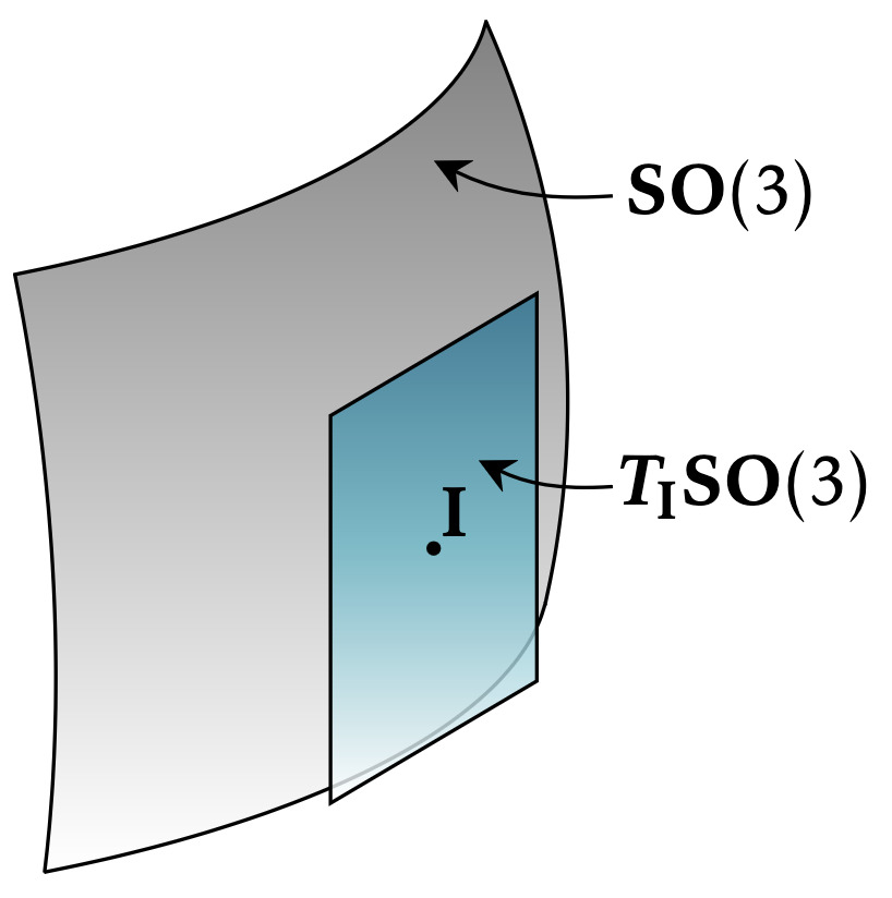
The same differentiation at $t = 0$ with $\mathbf{R}(0) = \mathbf{I}$ gives $\dot{\mathbf{R}}(0) \in \mathfrak{so}(3)$. A dimension count (six orthonormality constraints removed from nine entries) confirms equality of dimensions, so
\[T_{\mathbf{I}}\, SO(3) \;=\; \mathfrak{so}(3).\]In other words, the angular-velocity skew matrices are the tangent space at the identity, the role played by $\mathfrak{g} = T_{\mathbf{I}} G$ now realized for $G = SO(3)$.
The Lie algebra of $SO(3)$ is the three-dimensional real vector space of $3 \times 3$ skew-symmetric matrices $$\mathfrak{so}(3) \;:=\; \{ \mathbf{S} \in \mathbb{R}^{3\times 3} \,:\, \mathbf{S}^\top = -\mathbf{S} \} \;=\; T_{\mathbf{I}}\, SO(3),$$
$\color{blue}{\mathbf{Proof.}}$
Apply both sides to an arbitrary test vector $\mathbf{v} \in \mathbb{R}^3$ and use $[\boldsymbol{\omega}]\mathbf{v} = \boldsymbol{\omega} \times \mathbf{v}$ at each step:
\[\bigl[[\boldsymbol{\omega}_1], [\boldsymbol{\omega}_2]\bigr]\, \mathbf{v} \;=\; [\boldsymbol{\omega}_1][\boldsymbol{\omega}_2]\mathbf{v} - [\boldsymbol{\omega}_2][\boldsymbol{\omega}_1]\mathbf{v} \;=\; \boldsymbol{\omega}_1 \times (\boldsymbol{\omega}_2 \times \mathbf{v}) - \boldsymbol{\omega}_2 \times (\boldsymbol{\omega}_1 \times \mathbf{v}).\]Each triple cross product expands by the BAC-CAB identity $\mathbf{a} \times (\mathbf{b} \times \mathbf{c}) = \mathbf{b}(\mathbf{a} \cdot \mathbf{c}) - \mathbf{c}(\mathbf{a} \cdot \mathbf{b})$, after which the $\mathbf{v}(\boldsymbol{\omega}_1 \cdot \boldsymbol{\omega}_2)$ terms cancel:
\[\;=\; \bigl[\boldsymbol{\omega}_2(\boldsymbol{\omega}_1 \cdot \mathbf{v}) - \mathbf{v}(\boldsymbol{\omega}_1 \cdot \boldsymbol{\omega}_2)\bigr] - \bigl[\boldsymbol{\omega}_1(\boldsymbol{\omega}_2 \cdot \mathbf{v}) - \mathbf{v}(\boldsymbol{\omega}_1 \cdot \boldsymbol{\omega}_2)\bigr] \;=\; \boldsymbol{\omega}_2(\boldsymbol{\omega}_1 \cdot \mathbf{v}) - \boldsymbol{\omega}_1(\boldsymbol{\omega}_2 \cdot \mathbf{v}).\]The right-hand side is exactly $(\boldsymbol{\omega}_1 \times \boldsymbol{\omega}_2) \times \mathbf{v} = [\boldsymbol{\omega}_1 \times \boldsymbol{\omega}_2]\mathbf{v}$ by the vector triple-product identity $(\mathbf{a} \times \mathbf{b}) \times \mathbf{c} = (\mathbf{a} \cdot \mathbf{c})\mathbf{b} - (\mathbf{b} \cdot \mathbf{c})\mathbf{a}$. Since the equality holds for every $\mathbf{v}$, $\bigl[[\boldsymbol{\omega}_1], [\boldsymbol{\omega}_2]\bigr] = [\boldsymbol{\omega}_1 \times \boldsymbol{\omega}_2]$. $\blacksquare$
Exponential Coordinate Representation
A common motion encountered in robotics is the rotation of a body about a given axis by some amount. The link of a manipulator turns through a commanded angle about its joint axis, a hand reorients a grasped object by spinning it about an axis through the contact, and a quadrotor reorients itself by yawing about its body $z$-axis. The most natural parameterization of a three-dimensional rotation is given by a unit rotation axis $\hat{\boldsymbol{\omega}} \in \mathbb{R}^3$ together with a rotation angle $\theta \in \mathbb{R}$ about that axis. The fundamental problem is then to determine how this axis–angle representation can be mapped to a corresponding rotation matrix $\mathbf{R} \in SO(3)$.
Consider a body-fixed point $\mathbf{q}$ that rotates about the axis $\hat{\boldsymbol{\omega}}$ at unit angular speed. Then as we discussed, its instantaneous velocity is the tangential cross product:
\[\dot{\mathbf{q}}(t) \;=\; \hat{\boldsymbol{\omega}} \times \mathbf{q}(t) \;=\; [\hat{\boldsymbol{\omega}}]\, \mathbf{q}(t).\]This is a linear ODE in $\mathbb{R}^3$ with constant coefficient matrix $[\hat{\boldsymbol{\omega}}]$. Its unique solution with initial condition $\mathbf{q}(0) = \mathbf{q}_0$ is known as the matrix exponential applied to $\mathbf{q}_0$:
\[\mathbf{q}(t) \;=\; e^{[\hat{\boldsymbol{\omega}}]\, t}\, \mathbf{q}_0 \quad \text{where} \quad e^{\mathbf{M}} \;:=\; \sum_{k=0}^\infty \frac{\mathbf{M}^k}{k!}.\]The map $\mathbf{q}_0 \mapsto \mathbf{q}(t)$ is linear in $\mathbf{q}_0$, since multiplication by $e^{[\hat{\boldsymbol{\omega}}]\, t}$ is a linear operation. Geometrically this map carries each body-fixed point to its position after rotating for time $t$, which is exactly what the rotation matrix $\mathbf{R}(t)$ does to body-fixed points:
\[\mathbf{R}(t) \;=\; e^{[\hat{\boldsymbol{\omega}}]\, t}.\]At unit angular speed the time required to rotate by angle $\theta$ is $t = \theta$, so the finite rotation through angle $\theta$ about the axis $\hat{\boldsymbol{\omega}}$ is
\[\mathbf{R}(\hat{\boldsymbol{\omega}}, \theta) \;=\; e^{[\hat{\boldsymbol{\omega}}]\, \theta} \;=\; \sum_{k=0}^\infty \frac{([\hat{\boldsymbol{\omega}}]\, \theta)^k}{k!}.\]Encoding the axis and angle as a single vector $\boldsymbol{\omega} \;:=\; \theta\, \hat{\boldsymbol{\omega}} \;\in\; \mathbb{R}^3$, the formula shortens to $\mathbf{R} = \exp([\boldsymbol{\omega}])$, and the three components of $\boldsymbol{\omega}$ are the exponential coordinates of $\mathbf{R}$. The map $\exp : \mathfrak{so}(3) \to SO(3)$ sends a skew matrix in the tangent space at the identity to a rotation in the group;
Matrix Exponential on $SO(3)$: Rodrigues' Rotation Formula
So far the rotation $\mathbf{R} = e^{[\hat{\boldsymbol{\omega}}]\theta}$ exists only as an infinite series, which is exact but impractical to evaluate as written. Using the Taylor series, the infinite series for $e^{[\hat{\boldsymbol{\omega}}]\theta}$ collapses to a finite expression.
From the entries of $[\hat{\boldsymbol{\omega}}]$ together with $\Vert\hat{\boldsymbol{\omega}}\Vert = 1$, one can easily show that
\[[\hat{\boldsymbol{\omega}}]^2 \;=\; \hat{\boldsymbol{\omega}}\hat{\boldsymbol{\omega}}^\top - \mathbf{I}, \qquad [\hat{\boldsymbol{\omega}}]^3 \;=\; -[\hat{\boldsymbol{\omega}}],\]so higher powers cycle: $[\hat{\boldsymbol{\omega}}]^{2k+1} = (-1)^k [\hat{\boldsymbol{\omega}}]$ for odd indices, and $[\hat{\boldsymbol{\omega}}]^{2k+2} = (-1)^k [\hat{\boldsymbol{\omega}}]^2$ for even indices $\geq 2$. Splitting the series accordingly,
\[\begin{aligned} e^{[\hat{\boldsymbol{\omega}}]\theta} &= \mathbf{I} + \sum_{k=0}^\infty \frac{\theta^{2k+1}}{(2k+1)!} [\hat{\boldsymbol{\omega}}]^{2k+1} + \sum_{k=0}^\infty \frac{\theta^{2k+2}}{(2k+2)!} [\hat{\boldsymbol{\omega}}]^{2k+2} \\ &= \mathbf{I} + \underbrace{\left(\theta - \frac{\theta^3}{3!} + \frac{\theta^5}{5!} - \cdots\right)}_{\sin\theta}\, [\hat{\boldsymbol{\omega}}] + \underbrace{\left(\frac{\theta^2}{2!} - \frac{\theta^4}{4!} + \frac{\theta^6}{6!} - \cdots\right)}_{1 - \cos\theta}\, [\hat{\boldsymbol{\omega}}]^2 \\ &= \mathbf{I} + \sin\theta\, [\hat{\boldsymbol{\omega}}] + (1 - \cos\theta)\, [\hat{\boldsymbol{\omega}}]^2. \end{aligned}\]For a unit axis $\hat{\boldsymbol{\omega}} \in \mathbb{R}^3$ with $\Vert\hat{\boldsymbol{\omega}}\Vert = 1$ and angle $\theta \in \mathbb{R}$, $$ \boxed{\; e^{[\hat{\boldsymbol{\omega}}]\theta} \;=\; \mathbf{I} + \sin\theta\, [\hat{\boldsymbol{\omega}}] + (1 - \cos\theta)\, [\hat{\boldsymbol{\omega}}]^2 \;\in\; SO(3). \;} $$ For a general vector $\boldsymbol{\omega} \in \mathbb{R}^3$ with $\theta := \Vert\boldsymbol{\omega}\Vert$, $$ e^{[\boldsymbol{\omega}]} \;=\; \mathbf{I} + \frac{\sin\theta}{\theta}[\boldsymbol{\omega}] + \frac{1-\cos\theta}{\theta^2}[\boldsymbol{\omega}]^2. $$
The closed form makes orthogonality manifest: $\bigl(e^{[\hat{\boldsymbol{\omega}}]\theta}\bigr)^\top = e^{-[\hat{\boldsymbol{\omega}}]\theta} = \bigl(e^{[\hat{\boldsymbol{\omega}}]\theta}\bigr)^{-1}$ because $[\hat{\boldsymbol{\omega}}]^\top = -[\hat{\boldsymbol{\omega}}]$, and the determinant is pinned to $+1$ by continuity from $\det(\mathbf{I}) = 1$. So $e^{[\hat{\boldsymbol{\omega}}]\theta} \in SO(3)$ for every $(\hat{\boldsymbol{\omega}}, \theta)$.
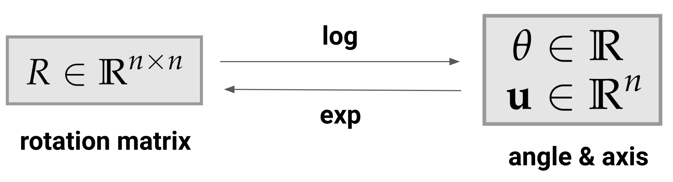
Matrix Logarithm on $SO(3)$: Euler's Rotation Theorem
Our next task is to show that for any rotation matrix $\mathbf{R} \in SO(3)$, one can always find a unit vector $\hat{\boldsymbol{\omega}}$ and a scalar $\theta$ such that $\mathbf{R} = e^{[\hat{\boldsymbol{\omega}}]\theta}$. Such a pair $(\hat{\boldsymbol{\omega}}, \theta)$ amounts to a matrix logarithm of $\mathbf{R}$, the inverse of the matrix exponential, written $\log(\mathbf{R}) = [\hat{\boldsymbol{\omega}}]\theta \in \mathfrak{so}(3)$. Where Rodrigues’ formula gives $\mathbf{R}$ from a pair $(\hat{\boldsymbol{\omega}}, \theta)$, the matrix logarithm recovers $(\hat{\boldsymbol{\omega}}, \theta)$ from $\mathbf{R}$.
Taking the trace of Rodrigues’ formula,
\[\operatorname{tr}(\mathbf{R}) \;=\; 1 + 2\cos\theta \;\Longrightarrow\; \theta \;=\; \cos^{-1}\!\left(\frac{\operatorname{tr}(\mathbf{R}) - 1}{2}\right) \,\in\, [0, \pi].\]For $\theta \neq 0, \pi$ the antisymmetric part of $\mathbf{R}$ yields the axis,
\[[\hat{\boldsymbol{\omega}}] \;=\; \frac{1}{2\sin\theta}\bigl(\mathbf{R} - \mathbf{R}^\top\bigr).\]Every $\mathbf{R} \in SO(3)$ therefore admits a representation $\mathbf{R} = e^{[\hat{\boldsymbol{\omega}}]\theta}$ for some unit axis $\hat{\boldsymbol{\omega}}$ and some $\theta \in [0, \pi]$.
Every $\mathbf{R} \in SO(3)$ is a rotation about some fixed unit axis $\hat{\boldsymbol{\omega}}$ through some angle $\theta \in [0, \pi]$. Equivalently, the exponential map $\exp : \mathfrak{so}(3) \to SO(3)$ is surjective.
Together, Rodrigues’ formula and the matrix logarithm give a way to move freely between $\mathfrak{so}(3)$ and $SO(3)$: the exponential takes an axis-angle pair to its rotation matrix, and the logarithm recovers axis and angle from any rotation. The two are inverses on a neighborhood of the identity, and Euler’s rotation theorem extends the exponential to a surjection onto the whole group.
Rigid Motions: $SE(3)$ and $\mathfrak{se}(3)$
Homogeneous Transformation Matrices and $SE(3)$
A rigid body in 3D has both an orientation $\mathbf{R} \in SO(3)$ and a position $\mathbf{p} \in \mathbb{R}^3$. The standard way to package both into a single algebraic object is the homogeneous transformation matrix, a $4 \times 4$ real matrix of the form
\[g \;=\; \begin{bmatrix} \mathbf{R} & \mathbf{p} \\ \mathbf{0}^\top & 1 \end{bmatrix},\]with the rotation $\mathbf{R}$ in the top-left $3 \times 3$ block, the translation $\mathbf{p}$ in the right column, and the row $(\mathbf{0}^\top, 1)$ at the bottom. The set of all such matrices is the special Euclidean group $SE(3)$, a six-dimensional smooth manifold (three coordinates for $\mathbf{R}$, three for $\mathbf{p}$).
The $4 \times 4$ size is dictated by the affine nature of rigid motion. The action of a configuration $T$ on a body-attached point $\mathbf{q}_b \in \mathbb{R}^3$, mapping it to its spatial-frame coordinates, is
\[\mathbf{q}_s \;=\; \mathbf{R}_{sb}\, \mathbf{q}_b + \mathbf{p}_{sb},\]a rotation followed by a translation. Padding the point to the homogeneous form $\bar{\mathbf{q}} = (\mathbf{q}^\top, 1)^\top \in \mathbb{R}^4$ turns this affine map into a linear map,
\[\bar{\mathbf{q}}_s \;=\; T_{sb}\, \bar{\mathbf{q}}_b,\]and composing two rigid motions reduces to plain $4 \times 4$ matrix multiplication. This matrix realization is what makes $SE(3)$ a Lie subgroup of $GL(4, \mathbb{R})$, and what lets the exponential machinery developed for $\mathfrak{so}(3)$ extend cleanly to rigid motions below.
The Special Euclidean group is $$ SE(3) := \left\{ T = \begin{bmatrix} \mathbf{R} & \mathbf{p} \\ \mathbf{0}^{\top} & 1 \end{bmatrix} \in \mathbb{R}^{4\times 4} : \mathbf{R} \in SO(3), \; \mathbf{p} \in \mathbb{R}^3 \right\}, $$ equipped with matrix multiplication as the group operation.
$SE(3)$ as a group
Specializing the group axioms to $SE(3)$ with matrix multiplication as the group operation:
- Closure. Given $T_1 = (\mathbf{R}_1, \mathbf{p}_1)$ and $T_2 = (\mathbf{R}_2, \mathbf{p}_2)$ in $SE(3)$, their product follows the chain rule for frames,
- Identity. $\mathbf{I}_4 \in SE(3)$, corresponding to $(\mathbf{R}, \mathbf{p}) = (\mathbf{I}, \mathbf{0})$.
- Inverse. The inverse takes a clean closed form,
- Associativity. Inherited from matrix multiplication.
Rigid motions preserve geometry. A homogeneous transformation $T = (\mathbf{R}, \mathbf{p}) \in SE(3)$ acts on a point $\mathbf{x} \in \mathbb{R}^3$ as $\mathbf{x} \mapsto \mathbf{R}\mathbf{x} + \mathbf{p}$. Using homogeneous coordinates $\bar{\mathbf{x}} = (\mathbf{x}^{\top}, 1)^{\top} \in \mathbb{R}^4$, this action is a single matrix multiplication,
\[T \bar{\mathbf{x}} \;=\; \begin{bmatrix} \mathbf{R} & \mathbf{p} \\ \mathbf{0}^{\top} & 1 \end{bmatrix} \begin{bmatrix} \mathbf{x} \\ 1 \end{bmatrix} \;=\; \begin{bmatrix} \mathbf{R}\mathbf{x} + \mathbf{p} \\ 1 \end{bmatrix},\]and by mild abuse of notation one writes $T\mathbf{x}$ for $\mathbf{R}\mathbf{x} + \mathbf{p}$. The action preserves both lengths and angles: for any $\mathbf{x}, \mathbf{y}, \mathbf{z} \in \mathbb{R}^3$,
\[\Vert T\mathbf{x} - T\mathbf{y} \Vert \;=\; \Vert \mathbf{x} - \mathbf{y} \Vert, \qquad \langle T\mathbf{x} - T\mathbf{z},\, T\mathbf{y} - T\mathbf{z} \rangle \;=\; \langle \mathbf{x} - \mathbf{z},\, \mathbf{y} - \mathbf{z} \rangle.\]Both follow from $\mathbf{R}^{\top}\mathbf{R} = \mathbf{I}$ once the translation cancels: $T\mathbf{x} - T\mathbf{y} = \mathbf{R}(\mathbf{x} - \mathbf{y})$, and the rotation-side preservation argument applies. If $\mathbf{x}, \mathbf{y}, \mathbf{z}$ are three vertices of a triangle, the transformed triangle ${T\mathbf{x}, T\mathbf{y}, T\mathbf{z}}$ is isometric to the original: same side lengths, same interior angles.
Twists and $\mathfrak{se}(3)$
A rigid body translating and rotating through space has at each instant a linear velocity $\mathbf{v} \in \mathbb{R}^3$ (rate of change of its position) and an angular velocity $\boldsymbol{\omega} \in \mathbb{R}^3$ (axis and rate of rotation, as for $SO(3)$). Packaging the two into a single 6-vector is the natural extension of the $\mathfrak{so}(3)$ story to $SE(3)$.
Concretely, let $T(t) \in SE(3)$ be a smooth trajectory written in block form
\[T(t) \;=\; \begin{bmatrix} \mathbf{R}(t) & \mathbf{p}(t) \\ \mathbf{0}^\top & 1 \end{bmatrix},\]so that, differentiating entry-by-entry and inverting block-wise,
\[\dot{T}(t) \;=\; \begin{bmatrix} \dot{\mathbf{R}}(t) & \dot{\mathbf{p}}(t) \\ \mathbf{0}^\top & 0 \end{bmatrix}, \qquad T^{-1}(t) \;=\; \begin{bmatrix} \mathbf{R}^{\top}(t) & -\mathbf{R}^{\top}(t)\mathbf{p}(t) \\ \mathbf{0}^\top & 1 \end{bmatrix}.\]Then we obtain
\[T^{-1}\dot{T} \;=\; \begin{bmatrix} \mathbf{R}^{\top} & -\mathbf{R}^{\top}\mathbf{p} \\ \mathbf{0}^\top & 1 \end{bmatrix} \begin{bmatrix} \dot{\mathbf{R}} & \dot{\mathbf{p}} \\ \mathbf{0}^\top & 0 \end{bmatrix} \;=\; \begin{bmatrix} \mathbf{R}^{\top}\dot{\mathbf{R}} & \mathbf{R}^{\top}\dot{\mathbf{p}} \\ \mathbf{0}^\top & 0 \end{bmatrix}.\]The top-left block is exactly the body angular velocity skew $[\boldsymbol{\omega}_b] := \mathbf{R}^{\top}\dot{\mathbf{R}}$ already identified in the $\mathfrak{so}(3)$ section, and the top-right block is the body linear velocity $\mathbf{v}_b := \mathbf{R}^{\top}\dot{\mathbf{p}} \in \mathbb{R}^3$. So at every $t$,
\[[\mathcal{V}_b] \;:=\; T^{-1}\dot{T} \;=\; \begin{bmatrix} [\boldsymbol{\omega}_b] & \mathbf{v}_b \\ \mathbf{0}^\top & 0 \end{bmatrix} \in \mathbb{R}^{4 \times 4}, \qquad \boldsymbol{\omega}, \mathbf{v} \in \mathbb{R}^3.\]The same construction with $T^{-1}$ multiplied on the right gives $\dot{T}\, T^{-1} \in \mathfrak{se}(3)$, with $\dot{\mathbf{R}}\mathbf{R}^{\top}$ in the angular block in place of $\mathbf{R}^{\top}\dot{\mathbf{R}}$. The two readings $T^{-1}\dot{T}$ and $\dot{T}\, T^{-1}$ are the body twist $[\mathcal{V}_b]$ and spatial twist $[\mathcal{V}_s]$ respectively; the distinction is developed in the section below.
This object is called a twist: it packages the linear and angular velocities of a rigid body into a single algebraic quantity, and the set of all such matrices forms the Lie algebra $\mathfrak{se}(3) = T_{\mathbf{I}} SE(3)$.
The Lie algebra of $SE(3)$ is the 6-dimensional real vector space $$ \mathfrak{se}(3) := \left\{ [\mathcal{V}] = \begin{bmatrix} [\boldsymbol{\omega}] & \mathbf{v} \\ \mathbf{0}^{\top} & 0 \end{bmatrix} : \mathbf{v} \in \mathbb{R}^3, \; [\boldsymbol{\omega}] \in \mathfrak{so}(3) \right\}. $$ The twist coordinates of $[\mathcal{V}]$ are the $6$-vector $$ \mathcal{V} = \begin{bmatrix} \boldsymbol{\omega} \\ \mathbf{v} \end{bmatrix} \in \mathbb{R}^6, $$
Physical interpretation of $\boldsymbol{\omega}$ and $\mathbf{v}$ depends on the choice of reference frame, taken up in the next section.
Spatial and Body Twists
A trajectory $T(t) \in SE(3)$ produces two natural elements of $\mathfrak{se}(3)$ by pre- and post-multiplying $\dot{T}$ by $T^{-1}$: the body twist $[\mathcal{V}_b] := T^{-1}\dot{T}$ and the spatial twist $[\mathcal{V}_s] := \dot{T}\, T^{-1}$, mirror images of each other. Block multiplication unpacks the two side by side as
\[[\mathcal{V}_b] = T^{-1}\dot{T} = \begin{bmatrix} \mathbf{R}^\top \dot{\mathbf{R}} & \mathbf{R}^\top \dot{\mathbf{p}} \\ \mathbf{0}^\top & 0 \end{bmatrix} = \begin{bmatrix} [\boldsymbol{\omega}_b] & \mathbf{v}_b \\ \mathbf{0}^\top & 0 \end{bmatrix}, \qquad [\mathcal{V}_s] = \dot{T}\, T^{-1} = \begin{bmatrix} \dot{\mathbf{R}}\mathbf{R}^\top & \dot{\mathbf{p}} - \dot{\mathbf{R}}\mathbf{R}^\top \mathbf{p} \\ \mathbf{0}^\top & 0 \end{bmatrix} = \begin{bmatrix} [\boldsymbol{\omega}_s] & \mathbf{v}_s \\ \mathbf{0}^\top & 0 \end{bmatrix},\]reading off the four components
\[[\boldsymbol{\omega}_b] = \mathbf{R}^\top \dot{\mathbf{R}}, \quad \mathbf{v}_b = \mathbf{R}^\top \dot{\mathbf{p}}, \qquad [\boldsymbol{\omega}_s] = \dot{\mathbf{R}}\mathbf{R}^\top, \quad \mathbf{v}_s = \dot{\mathbf{p}} - [\boldsymbol{\omega}_s]\,\mathbf{p}.\]These four quantities admit clear physical readings.
Body twist. Both components are direct. $\boldsymbol{\omega}_b$ is the angular velocity of the body expressed in body-frame coordinates. $\mathbf{v}_b = \mathbf{R}^\top \dot{\mathbf{p}}$ is the linear velocity of the body-frame origin expressed in body-frame coordinates: the spatial velocity $\dot{\mathbf{p}}$ rotated into body coordinates by $\mathbf{R}^\top$.
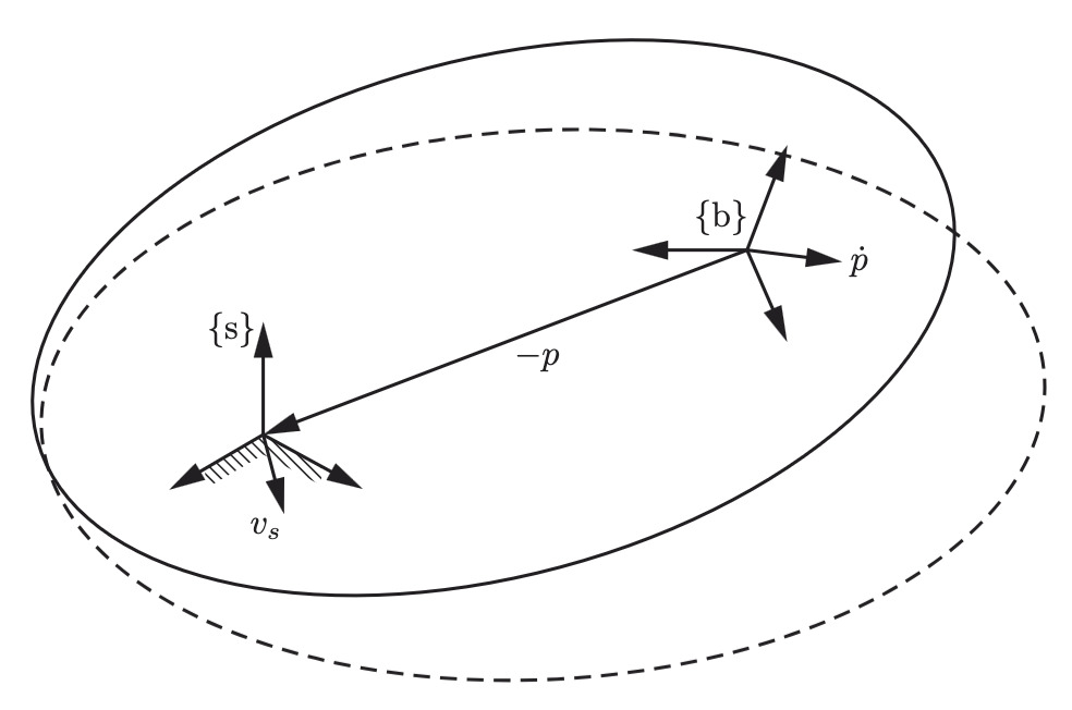
Spatial twist. $\boldsymbol{\omega}_s$ is the angular velocity of the body expressed in spatial-frame coordinates. The linear part $\mathbf{v}_s$ is more subtle since it is not the velocity of the body-frame origin in the spatial frame. Instead, rewrite
\[\mathbf{v}_s \;=\; \dot{\mathbf{p}} + \boldsymbol{\omega}_s \times (-\mathbf{p})\]and imagine the body extended infinitely as shown in the figure below. Then $\mathbf{v}_s$ is the spatial-frame velocity of the point on this extension currently at the spatial-frame origin.
Frame-independence. Analogously to angular velocities, the spatial twist \(\mathcal{V}_s\) does not depend on the choice of body frame \(\{b\}\), and the body twist \(\mathcal{V}_b\) does not depend on the choice of spatial frame \(\{s\}\). Replacing \(\{b\}\) with another body-fixed frame \(\{b'\}\) amounts to right-multiplying \(T_{sb}\) by a constant transformation \(T_{bb'}\) (constant since both frames are rigidly attached to the body):
\[\dot{T}_{sb'}\, T_{sb'}^{-1} \;=\; (\dot{T}_{sb}\, T_{bb'})\, (T_{sb}\, T_{bb'})^{-1} \;=\; \dot{T}_{sb}\, T_{bb'}\, T_{bb'}^{-1}\, T_{sb}^{-1} \;=\; \dot{T}_{sb}\, T_{sb}^{-1} \;=\; [\mathcal{V}_s].\]A symmetric calculation shows \([\mathcal{V}_b] = T_{sb}^{-1}\, \dot{T}_{sb}\) is unchanged under any constant change of the spatial frame.
$\mathbf{v}_s$ depends only on the rotation center, not on $\mathbf{p}$. The general formula
\[\mathbf{v}_s \;=\; \dot{\mathbf{p}} - \boldsymbol{\omega}_s \times \mathbf{p}\]takes the body-frame origin $\mathbf{p}$ and its velocity $\dot{\mathbf{p}}$ as inputs. When the motion is a pure rotation about a point $\mathbf{r}$ in space, the dependence on $\mathbf{p}$ vanishes entirely. Every body point $\mathbf{x}$ has velocity
\[\mathbf{u}(\mathbf{x}) \;=\; \boldsymbol{\omega}_s \times (\mathbf{x} - \mathbf{r}),\]so the body-frame origin, itself a body point, satisfies
\[\dot{\mathbf{p}} \;=\; \mathbf{u}(\mathbf{p}) \;=\; \boldsymbol{\omega}_s \times (\mathbf{p} - \mathbf{r}) \;=\; \boldsymbol{\omega}_s \times \mathbf{p} - \boldsymbol{\omega}_s \times \mathbf{r}.\]Substituting into the formula for $\mathbf{v}_s$, the $\boldsymbol{\omega}_s \times \mathbf{p}$ terms cancel,
\[\mathbf{v}_s \;=\; \underbrace{(\boldsymbol{\omega}_s \times \mathbf{p} - \boldsymbol{\omega}_s \times \mathbf{r})}_{\dot{\mathbf{p}}} - \boldsymbol{\omega}_s \times \mathbf{p} \;=\; -\boldsymbol{\omega}_s \times \mathbf{r}.\]The body-frame origin $\mathbf{p}$ drops out completely. Only the rotation center $\mathbf{r}$ survives, confirming that $\mathbf{v}_s$ is a property of the rigid motion’s spatial geometry, not of any particular choice of body frame.
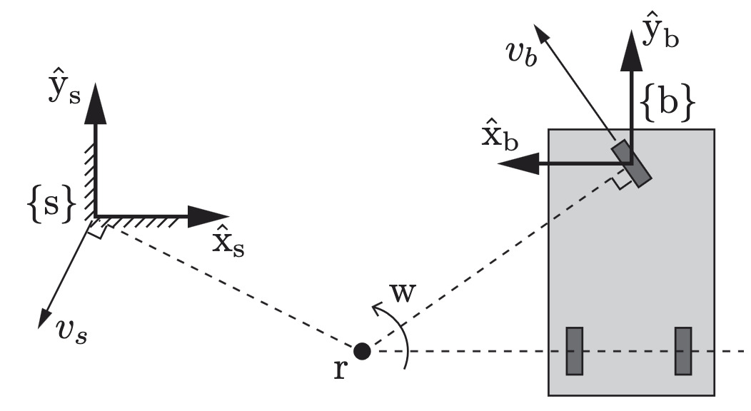
Consider a car (top view) whose chassis rotates instantaneously with angular speed $\omega = 2\,\mathrm{rad/s}$ about a point $\mathbf{r}$ in the plane, determined by the steering angle of its front wheel.
Frame Changes with Adjoint Representations
Spatial and body twists are two readings of the same instantaneous motion in different frames, so they must be related by a frame change. The same question arises in general: given a twist expressed in one frame, what 6-vector describes the same physical motion in another frame? This section gives the formula, taking the spatial-body relation as the entry point.
Spatial and body twists are linked by the algebraic identity
\[[\mathcal{V}_s] = \dot{T}\, T^{-1} \;=\; T\, (T^{-1}\, \dot{T})\, T^{-1} \;=\; T\, [\mathcal{V}_b]\, T^{-1},\]which displays the conjugation $T\, [\mathcal{V}_b]\, T^{-1}$:
\[T\, [\mathcal{V}_b]\, T^{-1} \;=\; \begin{bmatrix} \mathbf{R}\,[\boldsymbol{\omega}_b]\,\mathbf{R}^\top & \mathbf{R}\mathbf{v}_b - \mathbf{R}\,[\boldsymbol{\omega}_b]\,\mathbf{R}^\top \mathbf{p} \\ \mathbf{0}^\top & 0 \end{bmatrix},\]and using the $SO(3)$ identity $\mathbf{R}\,[\boldsymbol{\omega}]\,\mathbf{R}^\top = [\mathbf{R}\boldsymbol{\omega}]$ for the angular block, the corresponding 6-vector is
\[\mathcal{V}_s \;=\; \begin{bmatrix} \boldsymbol{\omega}_s \\ \mathbf{v}_s \end{bmatrix} \;=\; \begin{bmatrix} \mathbf{R} & \mathbf{0} \\ [\mathbf{p}]\,\mathbf{R} & \mathbf{R} \end{bmatrix} \begin{bmatrix} \boldsymbol{\omega}_b \\ \mathbf{v}_b \end{bmatrix} \;=\; \begin{bmatrix} \mathbf{R}\boldsymbol{\omega}_b \\ \mathbf{R}\mathbf{v}_b + \mathbf{p} \times \mathbf{R}\boldsymbol{\omega}_b \end{bmatrix}.\]The linear map $\mathcal{V}_b \mapsto \mathcal{V}_s$ on $\mathbb{R}^6$ is encoded by the $6 \times 6$ adjoint matrix.
For $T = (\mathbf{R}, \mathbf{p}) \in SE(3)$, the adjoint matrix $$ \operatorname{Ad}_T \;:=\; \begin{bmatrix} \mathbf{R} & \mathbf{0} \\ [\mathbf{p}]\,\mathbf{R} & \mathbf{R} \end{bmatrix} \;\in\; \mathbb{R}^{6 \times 6}. $$ transforms twists between frames via $\mathcal{V}_s = \operatorname{Ad}_T\, \mathcal{V}_b$, or equivalently $[\mathcal{V}_s] = T\, [\mathcal{V}_b]\, T^{-1}$. The same formula generalizes to any change of frame: given $T_{ab} \in SE(3)$ and a twist $\mathcal{V}$ expressed in frame $\{b\}$, its expression in frame $\{a\}$ is $\operatorname{Ad}_{T_{ab}}\, \mathcal{V}$.
The adjoint matrix has two clean algebraic properties that make it a frame-conversion calculus for twists. Both follow from direct block multiplication.
Composition. Chaining frame changes corresponds to multiplying their adjoint matrices:
\[\operatorname{Ad}_{T_1 T_2} \;=\; \operatorname{Ad}_{T_1} \operatorname{Ad}_{T_2}.\]If a twist is reexpressed first through $T_2$ and then through $T_1$, the combined frame change is given by the single adjoint $\operatorname{Ad}_{T_1 T_2}$. Multiplying transformations in $SE(3)$ becomes multiplying $6 \times 6$ matrices in the same order.
Inverse. Reversing a frame change is done by inverting the adjoint, which equals the adjoint of the inverse transformation:
\[(\operatorname{Ad}_T)^{-1} \;=\; \operatorname{Ad}_{T^{-1}} \;=\; \begin{bmatrix} \mathbf{R}^\top & \mathbf{0} \\ -\mathbf{R}^\top [\mathbf{p}] & \mathbf{R}^\top \end{bmatrix}.\]If \(\mathcal{V}_a = \operatorname{Ad}_T\, \mathcal{V}_b\) converts a twist from \(\{b\}\) to \(\{a\}\), then \(\mathcal{V}_b = \operatorname{Ad}_{T^{-1}}\, \mathcal{V}_a\) converts back.
Together the two identities say that the map $T \mapsto \operatorname{Ad}_T$ is a group representation of $SE(3)$: every frame change of twists is encoded by some $6 \times 6$ matrix, and these matrices multiply and invert the same way the underlying $T$s do. This is the algebraic bedrock of geometric formulations of the manipulator Jacobian and Newton-Euler dynamics, where twists move freely between frames without ad-hoc reindexing.
Screws: a Geometric Description of Twists
Just as an angular velocity $\boldsymbol{\omega}$ can be viewed as $\hat{\boldsymbol{\omega}}\,\dot{\theta}$, where $\hat{\boldsymbol{\omega}}$ is the unit rotation axis and $\dot{\theta}$ is the rate of rotation about that axis, a twist $\mathcal{V}$ admits the analogous decomposition
\[\mathcal{V} \;=\; \mathcal{S}\, \dot{\theta},\]where $\mathcal{S}$ is a 6-vector called the screw axis and $\dot{\theta}$ is a scalar rate of motion about it. The screw axis generalizes the unit rotation axis from $SO(3)$ to $SE(3)$: it encodes both an axis line in space and a pitch describing how much translation accompanies each radian of rotation about that line.
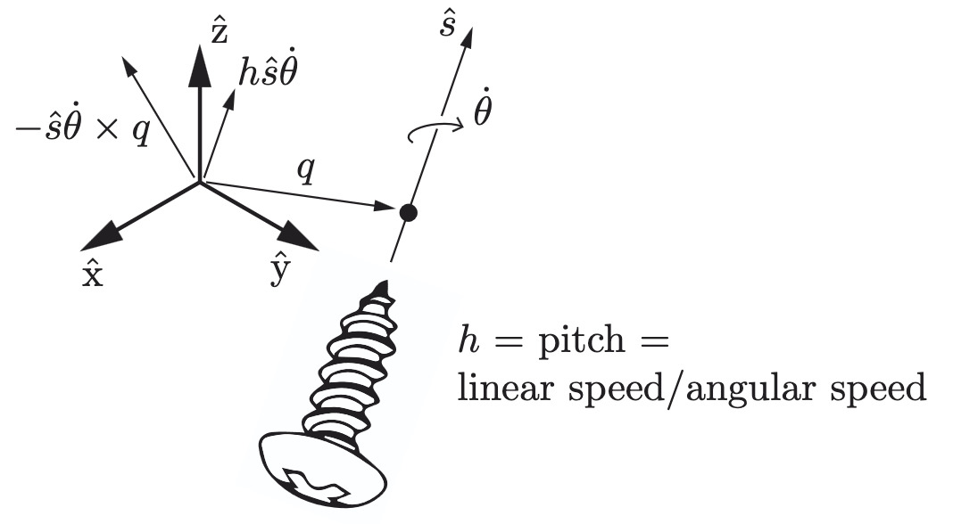
Geometrically, this is the content of the theorem of Mozzi (1763) and Chasles (1830): every rigid motion is a screw motion, a simultaneous rotation about a directed line in space and translation along that same line, like turning a corkscrew. The line is the screw’s axis, the linear distance per radian of rotation is its pitch, and the scalar amount of motion is its magnitude $\theta$. To turn this geometric picture into algebra, we collect the axis direction, the location of the axis, and the pitch into a single normalized 6-vector $\mathcal{S}$.
A screw axis is the geometric data of a directed line in space together with a pitch. For a rotational screw motion, it consists of
- any point $\mathbf{q} \in \mathbb{R}^3$ on the axis,
- a unit direction $\hat{\mathbf{s}} \in \mathbb{R}^3$ along the axis, $\Vert\hat{\mathbf{s}}\Vert = 1$,
- a pitch $h \in \mathbb{R}$, the translation along the axis per radian of rotation about it.
Matrix form and frame change
Since a screw axis is just a normalized twist, it inherits the algebraic structure of $\mathfrak{se}(3)$. Writing $\mathcal{S} = (\boldsymbol{\omega}, \mathbf{v})$ in components, with $\boldsymbol{\omega} = (\omega_1, \omega_2, \omega_3) \in \mathbb{R}^3$ the angular part and $\mathbf{v} \in \mathbb{R}^3$ the linear part, the $4 \times 4$ matrix representation is
\[[\mathcal{S}] \;=\; \begin{bmatrix} [\boldsymbol{\omega}] & \mathbf{v} \\ \mathbf{0}^\top & 0 \end{bmatrix} \;\in\; \mathfrak{se}(3), \qquad [\boldsymbol{\omega}] \;=\; \begin{bmatrix} 0 & -\omega_3 & \omega_2 \\ \omega_3 & 0 & -\omega_1 \\ -\omega_2 & \omega_1 & 0 \end{bmatrix} \;\in\; \mathfrak{so}(3),\]with the bottom row of $[\mathcal{S}]$ all zero.
A change of frame transforms a screw axis by the adjoint, exactly as for any twist. If \(\mathcal{S}_a\) and \(\mathcal{S}_b\) are its representations in frames \(\{a\}\) and \(\{b\}\), and \(T_{ab}, T_{ba} = T_{ab}^{-1} \in SE(3)\) are the relative configurations,
\[\mathcal{S}_a \;=\; \operatorname{Ad}_{T_{ab}}\,\mathcal{S}_b, \qquad \mathcal{S}_b \;=\; \operatorname{Ad}_{T_{ba}}\,\mathcal{S}_a.\]Recovering the screw data from a twist
Given an arbitrary twist $\mathcal{V} = (\boldsymbol{\omega}, \mathbf{v}) \in \mathbb{R}^6$, the four pieces of screw data $(\hat{\mathbf{s}}, \mathbf{q}, h, \dot{\theta})$ are read off directly. For $\boldsymbol{\omega} \neq \mathbf{0}$ (a screw with finite pitch),
\[\hat{\mathbf{s}} \;=\; \frac{\boldsymbol{\omega}}{\Vert\boldsymbol{\omega}\Vert}, \qquad \dot{\theta} \;=\; \Vert\boldsymbol{\omega}\Vert, \qquad h \;=\; \frac{\boldsymbol{\omega}^\top \mathbf{v}}{\Vert\boldsymbol{\omega}\Vert^2}, \qquad \mathbf{q} \;=\; \frac{\boldsymbol{\omega} \times \mathbf{v}}{\Vert\boldsymbol{\omega}\Vert^2}.\]The first two come from normalizing $\boldsymbol{\omega}$: the unit direction $\hat{\mathbf{s}}$ is the axis of rotation, and $\dot{\theta} = \Vert\boldsymbol{\omega}\Vert$ is the angular speed about it. The pitch and the axis point come from projecting $\mathbf{v}$ along and across $\hat{\mathbf{s}}$. Throughout, substitute the Definition’s expressions
\[\boldsymbol{\omega} \;=\; \hat{\mathbf{s}}\,\dot{\theta}, \qquad \mathbf{v} \;=\; \bigl(-\hat{\mathbf{s}} \times \mathbf{q} + h\,\hat{\mathbf{s}}\bigr)\,\dot{\theta}.\]For $h$, take the inner product with $\boldsymbol{\omega}$:
\[\begin{aligned} \boldsymbol{\omega}^\top \mathbf{v} &\;=\; (\hat{\mathbf{s}}\,\dot{\theta})^\top \bigl(-\hat{\mathbf{s}} \times \mathbf{q} + h\,\hat{\mathbf{s}}\bigr)\,\dot{\theta} \\ &\;=\; \dot{\theta}^2\bigl[\,{-\hat{\mathbf{s}}^\top(\hat{\mathbf{s}} \times \mathbf{q})} + h\,\hat{\mathbf{s}}^\top \hat{\mathbf{s}}\,\bigr] \\ &\;=\; \dot{\theta}^2 \cdot h && \bigl(\hat{\mathbf{s}}^\top(\hat{\mathbf{s}} \times \mathbf{q}) = 0,\ \ \Vert\hat{\mathbf{s}}\Vert = 1\bigr) \\ &\;=\; h\,\Vert\boldsymbol{\omega}\Vert^2. \end{aligned}\]For $\mathbf{q}$, take the cross product with $\boldsymbol{\omega}$:
\[\begin{aligned} \boldsymbol{\omega} \times \mathbf{v} &\;=\; (\hat{\mathbf{s}}\,\dot{\theta}) \times \bigl(-\hat{\mathbf{s}} \times \mathbf{q} + h\,\hat{\mathbf{s}}\bigr)\,\dot{\theta} \\ &\;=\; -\dot{\theta}^2\, \hat{\mathbf{s}} \times (\hat{\mathbf{s}} \times \mathbf{q}) && (\hat{\mathbf{s}} \times \hat{\mathbf{s}} = 0) \\ &\;=\; -\dot{\theta}^2\,\bigl[(\hat{\mathbf{s}}^\top\mathbf{q})\,\hat{\mathbf{s}} - \mathbf{q}\bigr] && (\text{vector triple product}) \\ &\;=\; \Vert\boldsymbol{\omega}\Vert^2\,\bigl(\mathbf{q} - (\hat{\mathbf{s}}^\top\mathbf{q})\,\hat{\mathbf{s}}\bigr). \end{aligned}\]The right-hand side is $\Vert\boldsymbol{\omega}\Vert^2$ times the perpendicular component of $\mathbf{q}$ relative to $\hat{\mathbf{s}}$, geometrically the foot of the perpendicular dropped from the spatial origin onto the axis line, i.e., the point on the axis nearest the origin. The definition allowed any point on the axis to play $\mathbf{q}$; dividing through fixes this canonical one, $\mathbf{q} = (\boldsymbol{\omega} \times \mathbf{v})/\Vert\boldsymbol{\omega}\Vert^2$.
When $\boldsymbol{\omega} = \mathbf{0}$ (pure translation, infinite pitch) there is no axis location to recover, and one normalizes the linear part instead,
\[\hat{\mathbf{s}} \;=\; \frac{\mathbf{v}}{\Vert\mathbf{v}\Vert}, \qquad \dot{\theta} \;=\; \Vert\mathbf{v}\Vert.\]Revolute and prismatic joints
Two extreme values of the pitch occupy distinguished places in elementary robotics, since each corresponds to one of the two basic joint types:
- A zero-pitch screw ($h = 0$) gives pure rotation about $\ell$ with no translation. The twist reduces to $(\hat{\mathbf{s}}, -\hat{\mathbf{s}} \times \mathbf{q})$, the velocity of a revolute joint.
- An infinite-pitch screw gives pure translation along $\ell$ with no rotation. The twist reduces to $(\mathbf{0}, \hat{\mathbf{v}})$, the velocity of a prismatic joint.
The screw axis $\mathcal{S}$ is exactly the classical screw of Ball (1900) [3]: its first three components specify a unit direction along the axis, and the last three encode the axis location and the pitch in a single 6-vector. The rigid motion generated by following $\mathcal{S}$ for magnitude $\theta$ is the matrix exponential $T = e^{[\mathcal{S}]\theta} \in SE(3)$, derived in closed form in the next section.
The three-wheeled vehicle worked out in the previous section has spatial twist $$\mathcal{V}_s \;=\; \bigl(\boldsymbol{\omega}_s, \mathbf{v}_s\bigr) \;=\; \bigl((0, 0, 2),\; (-2, -4, 0)\bigr).$$ Read off pitch and axis: $$h \;=\; \frac{\boldsymbol{\omega}_s^\top \mathbf{v}_s}{\Vert\boldsymbol{\omega}_s\Vert^2} \;=\; \frac{0}{4} \;=\; 0, \qquad \mathbf{q}^* \;=\; \frac{\boldsymbol{\omega}_s \times \mathbf{v}_s}{\Vert\boldsymbol{\omega}_s\Vert^2} \;=\; \frac{(8, -4, 0)}{4} \;=\; (2, -1, 0).$$ Pitch is zero (pure rotation), and the recovered axis point matches the rotation center $\mathbf{r}_s = (2, -1, 0)$ from the original setup. Normalizing the twist gives the screw axis $$\mathcal{S} \;=\; \frac{\mathcal{V}_s}{\Vert\boldsymbol{\omega}_s\Vert} \;=\; \frac{1}{2}\, \bigl((0, 0, 2),\, (-2, -4, 0)\bigr) \;=\; \bigl((0, 0, 1),\, (-1, -2, 0)\bigr),$$ with rate $\dot{\theta} = \Vert\boldsymbol{\omega}_s\Vert = 2\,\mathrm{rad/s}$. Verification: $\mathcal{S}\,\dot{\theta} = ((0,0,1),(-1,-2,0)) \cdot 2 = ((0,0,2),(-2,-4,0)) = \mathcal{V}_s$.
Exponential Coordinate Representation: Chasles-Mozzi Theorem
Just as a rotation about an axis by an angle $\theta$ is parameterized by $(\hat{\boldsymbol{\omega}},\theta)$ and mapped to a rotation matrix $\mathbf R\in SO(3)$, a screw motion is parameterized by a screw axis $\mathcal{S}$ and a scalar displacement $\theta$, and mapped to a rigid transformation $T\in SE(3)$. The goal is to determine this map.
Consider a body-fixed point $\bar{\mathbf{q}}_0 \in \mathbb{R}^4$ in homogeneous coordinates that moves rigidly with the body. Its trajectory $\bar{\mathbf{q}}(t) = T(t)\,\bar{\mathbf{q}}_0$ satisfies the kinematic equation
\[\dot{\bar{\mathbf{q}}}(t) = \dot{T}(t)\,\bar{\mathbf{q}}_0 = \dot{T}(t) T^{-1}(t) \,\bar{\mathbf{q}}(t) = [\mathcal{V}]\,\bar{\mathbf{q}}(t),\]a linear ODE in $\mathbb{R}^4$ with constant coefficient matrix $[\mathcal{V}]$ when the twist is held constant. Its unique solution is the matrix exponential applied to $\bar{\mathbf{q}}_0$,
\[\bar{\mathbf{q}}(t) \;=\; e^{[\mathcal{V}]\,t}\,\bar{\mathbf{q}}_0, \quad \text{where} \quad e^{\mathbf{M}} \;:=\; \sum_{k=0}^\infty \frac{\mathbf{M}^k}{k!}.\]Since the same transformation acts on every body-fixed point,
\[T(t) \;=\; e^{[\mathcal{V}]\,t} \;\in\; SE(3).\]At unit speed, a displacement of magnitude $\theta$ along the screw axis $\mathcal{S}$ is therefore
\[T(\mathcal{S}, \theta) \;=\; e^{[\mathcal{S}]\theta} \;=\; \sum_{k=0}^\infty \frac{([\mathcal{S}]\,\theta)^k}{k!}.\]The 6-vector $\mathcal{S}\theta \in \mathbb{R}^6$ is called the exponential coordinates of $T$, directly generalizing the axis-angle coordinates $\hat{\boldsymbol\omega}\theta\in\mathbb R^3$ on $SO(3)$.
Matrix Exponential on $SE(3)$: Closed Form
Just as Rodrigues’ formula provides a closed form for the exponential map on $SO(3)$, the exponential map on $SE(3)$ also admits a closed form. The derivation exploits the block-triangular structure of the twist matrix $e^{[\mathcal{S}]t}$.
Write the rigid motion in block form
\[T(t) = \begin{bmatrix} \mathbf{R}(t) & \mathbf{p}(t) \\ \mathbf{0}^\top & 1 \end{bmatrix},\]with $\mathbf{R}(0) = \mathbf{I}$ and $\mathbf{p}(0) = \mathbf{0}$. Substituting into $\dot{T} = [\mathcal{S}]\,T$ expands block-by-block into
\[\dot{\mathbf{R}}(t) \;=\; [\boldsymbol{\omega}]\,\mathbf{R}(t), \qquad \dot{\mathbf{p}}(t) \;=\; [\boldsymbol{\omega}]\,\mathbf{p}(t) + \mathbf{v}.\]The rotational equation is the $SO(3)$ kinematic ODE; its solution is $\mathbf{R}(\theta) = e^{[\boldsymbol{\omega}]\theta}$, with closed form given by Rodrigues’ formula. For the translational equation, multiply both sides by the integrating factor $e^{-[\boldsymbol{\omega}]t}$ to fold the homogeneous part into a total derivative,
\[\frac{d}{dt}\bigl(e^{-[\boldsymbol{\omega}]t}\,\mathbf{p}(t)\bigr) \;=\; e^{-[\boldsymbol{\omega}]t}\,\mathbf{v} \Rightarrow \mathbf{p}(\theta) \;=\; \int_0^\theta e^{[\boldsymbol{\omega}](\theta - s)}\,\mathbf{v}\, ds.\]Integrating from $0$ to $\theta$ with $\mathbf{p}(0) = \mathbf{0}$ and multiplying back by $e^{[\boldsymbol{\omega}]\theta}$ gives
\[\mathbf{p}(\theta) \;=\; \int_0^\theta e^{[\boldsymbol{\omega}](\theta - s)}\,\mathbf{v}\, ds.\]The substitution $u = \theta - s$ pulls $\mathbf{v}$ out of the integral as a matrix-vector product,
\[\mathbf{p}(\theta) \;=\; G(\theta)\,\mathbf{v}, \qquad G(\theta) \;:=\; \int_0^\theta e^{[\boldsymbol{\omega}]s}\,ds.\]The closed form of $G(\theta)$ splits into two cases. For $\Vert\boldsymbol{\omega}\Vert = 1$ (finite pitch), substituting Rodrigues’ formula and integrating term-by-term,
\[G(\theta) \;=\; \int_0^\theta \bigl(\mathbf{I} + \sin s\,[\boldsymbol{\omega}] + (1 - \cos s)\,[\boldsymbol{\omega}]^2\bigr)\,ds \;=\; \mathbf{I}\theta + (1-\cos\theta)\,[\boldsymbol{\omega}] + (\theta - \sin\theta)\,[\boldsymbol{\omega}]^2.\]For $\boldsymbol{\omega} = \mathbf{0}$ (infinite pitch), the integrand reduces to $\mathbf{I}$, so $G(\theta) = \mathbf{I}\theta$ and $\mathbf{R}(\theta) = \mathbf{I}$, and the full exponential collapses to $e^{[\mathcal{S}]\theta} = \mathbf{I} + [\mathcal{S}]\theta$. Combining the rotation and translation blocks gives the closed-form $SE(3)$ counterpart of Rodrigues’ formula.
For a screw axis $\mathcal{S} = (\boldsymbol{\omega}, \mathbf{v}) \in \mathbb{R}^6$ and $\theta \in \mathbb{R}$, the matrix exponential of $[\mathcal{S}]\theta \in \mathfrak{se}(3)$ takes one of two forms.
- Case 1 ($\Vert\boldsymbol{\omega}\Vert = 1$, finite pitch): $$ \boxed{\; e^{[\mathcal{S}]\theta} \;=\; \begin{bmatrix} e^{[\boldsymbol{\omega}]\theta} & G(\theta)\,\mathbf{v} \\ \mathbf{0}^\top & 1 \end{bmatrix} \in SE(3), \;} $$ where the rotation block is Rodrigues' formula $$e^{[\boldsymbol{\omega}]\theta} \;=\; \mathbf{I} + \sin\theta\,[\boldsymbol{\omega}] + (1-\cos\theta)\,[\boldsymbol{\omega}]^2,$$ and the integrator matrix is $$G(\theta) \;=\; \mathbf{I}\theta + (1-\cos\theta)\,[\boldsymbol{\omega}] + (\theta-\sin\theta)\,[\boldsymbol{\omega}]^2.$$
- Case 2 ($\boldsymbol{\omega} = \mathbf{0}$ and $\Vert\mathbf{v}\Vert = 1$, infinite pitch): $$ \boxed{\; e^{[\mathcal{S}]\theta} \;=\; \begin{bmatrix} \mathbf{I} & \mathbf{v}\theta \\ \mathbf{0}^\top & 1 \end{bmatrix}. \;} $$
The translation block $G(\theta)\,\mathbf{v}$ is the integral of the rotation $e^{[\boldsymbol{\omega}]s}$ against the linear part $\mathbf{v}$. Its three terms have direct geometric content: $\mathbf{I}\theta\,\mathbf{v}$ is the straight slide along $\mathbf{v}$, $(1-\cos\theta)[\boldsymbol{\omega}]\,\mathbf{v}$ adds the circular component perpendicular to $\boldsymbol{\omega}$ swept out by points off the axis, and $(\theta - \sin\theta)[\boldsymbol{\omega}]^2\,\mathbf{v}$ corrects the along-axis component to give the screw advance per radian of rotation.
Matrix Logarithm on $SE(3)$: Chasles-Mozzi Theorem
Our next task is to show that for any $T \in SE(3)$, one can always find a screw axis $\mathcal{S}$ and a scalar $\theta$ such that $T = e^{[\mathcal{S}]\theta}$. The rotational block determines $(\hat{\omega},\theta)$ through the $SO(3)$ matrix logarithm,
\[R=e^{[\hat{\omega}]\theta}.\]The translational block then determines $\mathbf{v}$ through $\mathbf{v} = G^{-1}(\theta)\,\mathbf{p}$. To compute $G^{-1}(\theta)$ in closed form, look for an inverse in the same basis ${\mathbf{I}, [\hat{\boldsymbol{\omega}}], [\hat{\boldsymbol{\omega}}]^2}$,
\[G^{-1}(\theta) \;=\; a\,\mathbf{I} + b\,[\hat{\boldsymbol{\omega}}] + c\,[\hat{\boldsymbol{\omega}}]^2,\]with scalar coefficients $a, b, c$ to be determined. Because $\hat{\boldsymbol{\omega}}$ is a unit vector, repeated cross products close back: $[\hat{\boldsymbol{\omega}}]^3 = -[\hat{\boldsymbol{\omega}}]$ and $[\hat{\boldsymbol{\omega}}]^4 = -[\hat{\boldsymbol{\omega}}]^2$. Expanding $G(\theta)\,G^{-1}(\theta)$ and reducing every term to $\mathbf{I}, [\hat{\boldsymbol{\omega}}], [\hat{\boldsymbol{\omega}}]^2$ gives
\[\begin{aligned} G(\theta)\,G^{-1}(\theta) \;=\; & \theta a\,\mathbf{I} \;+\; \bigl[b\sin\theta + (a-c)(1-\cos\theta)\bigr]\,[\hat{\boldsymbol{\omega}}] \\ & \;+\; \bigl[c\sin\theta + b(1-\cos\theta) + a(\theta - \sin\theta)\bigr]\,[\hat{\boldsymbol{\omega}}]^2. \end{aligned}\]Setting this equal to $\mathbf{I}$ matches three scalar equations,
\[\begin{aligned} \theta a &\;=\; 1, \\ b\sin\theta + (a-c)(1-\cos\theta) &\;=\; 0, \\ c\sin\theta + b(1-\cos\theta) + a(\theta - \sin\theta) &\;=\; 0. \end{aligned}\]Solving the linear system in $(a, b, c)$, with the half-angle identity $\sin\theta/(1-\cos\theta) = \cot(\theta/2)$ collapsing the trigonometric ratios, gives the closed form
\[\boxed{\;G^{-1}(\theta) \;=\; \frac{1}{\theta}\,\mathbf{I} \;-\; \frac{1}{2}\,[\hat{\boldsymbol{\omega}}] \;+\; \left(\frac{1}{\theta} \;-\; \frac{1}{2}\cot\frac{\theta}{2}\right)[\hat{\boldsymbol{\omega}}]^2,\;}\]valid for $\theta \in (0, 2\pi)$, where $G(\theta)$ is invertible.
The boundary case $\mathbf{R} = \mathbf{I}$ is pure translation, handled directly by $[\mathcal{V}] = \begin{bmatrix} \mathbf{0} & \mathbf{p}/\Vert\mathbf{p}\Vert ; \mathbf{0}^\top & 0 \end{bmatrix}$ with $\omega = 0$, $\mathbf{v} = \mathbf{p} / \Vert\mathbf{p}\Vert$, and $\theta = \Vert\mathbf{p}\Vert$.
In other words, every rigid motion is generated by a single screw axis. Rotation and translation are not independent primitives but two aspects of the same geometric object. This observation is the content of the Chasles–Mozzi theorem.
For any $T \in SE(3)$, there exist a screw axis $\mathcal{S}$ and a scalar $\theta$ such that $$T \;=\; e^{[\mathcal{S}]\theta}.$$ Equivalently, the exponential map $\exp : \mathfrak{se}(3) \to SE(3)$ is surjective. Every rigid-body displacement can therefore be represented as a motion about a single fixed screw axis. The pair $(\mathcal{S},\theta)$ provides the natural coordinate system for $SE(3)$, just as axis-angle coordinates do for $SO(3)$.
Together, the matrix exponential and logarithm provide a complete bridge between $\mathfrak{se}(3)$ and $SE(3)$. They play for rigid motions exactly the role that Rodrigues’ formula and Euler’s rotation theorem play for rotations, unifying translation and rotation under the single geometric primitive of the screw.
Wrenches
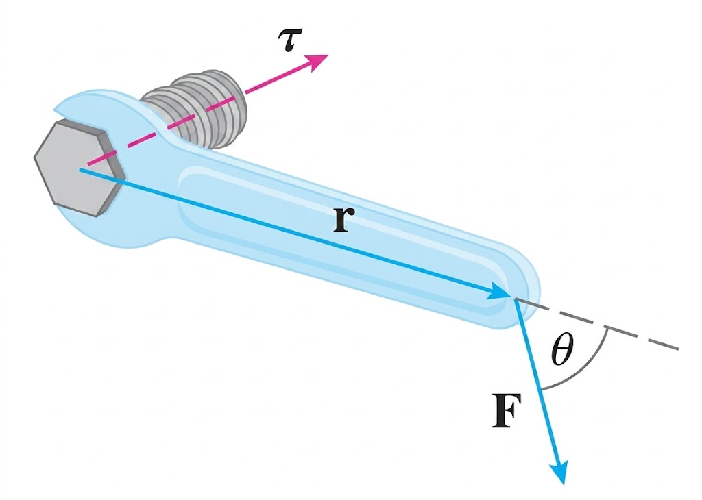
When a mechanical wrench is applied to a bolt (Fig 19), a linear force $\mathbf{f}$ at the end of the wrench handle produces a turning effect about the bolt axis: a moment
\[\boldsymbol{\tau} \;=\; \mathbf{r} \times \mathbf{f},\]where $\mathbf{r} \in \mathbb{R}^3$ is the position of the force application point relative to the bolt center. The magnitude $\Vert\boldsymbol{\tau}\Vert = \Vert\mathbf{r}\Vert\,\Vert\mathbf{f}\Vert\sin\theta$ grows with the lever arm $\Vert\mathbf{r}\Vert$, which is why a longer-handled wrench loosens a tight bolt more easily. The full mechanical effect of the applied force is the pair $(\boldsymbol{\tau}, \mathbf{f})$: a moment about the bolt center together with a residual linear force.
Packaging this pair into a single 6-vector gives the wrench, the dual of the twist: the two 6-vectors are paired by an inner product $\mathcal{V}^\top \mathcal{F}$ that measures instantaneous power, and they transform between frames by contragredient laws, twists by the adjoint and wrenches by its transpose.
A wrench is a 6-vector $\mathcal{F} = (\boldsymbol{\tau}, \mathbf{f}) \in \mathbb{R}^6$ where $\boldsymbol{\tau} \in \mathbb{R}^3$ is a moment and $\mathbf{f} \in \mathbb{R}^3$ is a linear force, both measured in the same reference frame and both referred to the origin of that frame, $$ \mathcal{F} \;=\; \begin{bmatrix} \boldsymbol{\tau} \\ \mathbf{f} \end{bmatrix} \;\in\; \mathbb{R}^6. $$ Expressing the wrench in the spatial frame $\{s\}$ gives the spatial wrench $\mathcal{F}_s$, and in the body frame $\{b\}$ gives the body wrench $\mathcal{F}_b$.
Power: the twist-wrench pairing
The instantaneous power delivered by a wrench $\mathcal{F}$ to a body moving with twist $\mathcal{V}$ is the inner product
\[\delta W \;=\; \mathcal{V}^\top \mathcal{F} \;=\; \boldsymbol{\omega} \cdot \boldsymbol{\tau} + \mathbf{v} \cdot \mathbf{f},\]provided both are expressed in the same frame. Power is a physically measurable scalar quantity, so it cannot depend on the frame in which it is computed:
\[\mathcal{V}_s^\top \mathcal{F}_s \;=\; \mathcal{V}_b^\top \mathcal{F}_b.\]Frame transformation: the contragredient adjoint
This frame-invariance of power is the defining algebraic property of the twist-wrench pairing, and it determines how wrenches transform between frames. Substituting the known twist transformation \(\mathcal{V}_s = \operatorname{Ad}_{T_{sb}}\, \mathcal{V}_b\) into the invariance identity,
\[\mathcal{V}_b^\top \mathcal{F}_b \;=\; \mathcal{V}_s^\top \mathcal{F}_s \;=\; (\operatorname{Ad}_{T_{sb}}\, \mathcal{V}_b)^\top \mathcal{F}_s \;=\; \mathcal{V}_b^\top \operatorname{Ad}_{T_{sb}}^\top \mathcal{F}_s.\]Since this must hold for every \(\mathcal{V}_b \in \mathbb{R}^6\), the two sides force
\[\boxed{\;\mathcal{F}_b \;=\; \operatorname{Ad}_{T_{sb}}^\top\, \mathcal{F}_s.\;}\]Twists transform by \(\operatorname{Ad}_{T_{sb}}\), wrenches by \(\operatorname{Ad}_{T_{sb}}^\top\); the two transformation laws are contragredient, and their product (power) is the invariant. Algebraically, \(\mathcal{F}\) lives in the dual space \(\mathfrak{se}(3)^*\) of \(\mathfrak{se}(3)\), on which the adjoint acts by its transpose.
Summary
We have introduced the modern, Lie-theoretic formulation of rigid-body motion. The objects, identities, and frame-change rules are collected below.
$SO(3)$ and $\mathfrak{so}(3)$
The matrix Lie group of orientations and its Lie algebra of $3 \times 3$ skew-symmetric matrices, identified with $\mathbb{R}^3$ via the hat operator $[\boldsymbol{\omega}]\,\mathbf{v} = \boldsymbol{\omega} \times \mathbf{v}$.
\[\mathbf{R} \in SO(3) \iff \mathbf{R}^\top \mathbf{R} = \mathbf{I},\;\det \mathbf{R} = 1, \qquad [\boldsymbol{\omega}] = \begin{pmatrix} 0 & -\omega_3 & \omega_2 \\ \omega_3 & 0 & -\omega_1 \\ -\omega_2 & \omega_1 & 0 \end{pmatrix} \in \mathfrak{so}(3).\]Kinematics and Rodrigues’ formula ($\Vert\boldsymbol{\omega}\Vert = 1$):
\[\dot{\mathbf{R}} = \mathbf{R}\,[\boldsymbol{\omega}_b] = [\boldsymbol{\omega}_s]\,\mathbf{R}, \qquad e^{[\boldsymbol{\omega}]\theta} = \mathbf{I} + \sin\theta\,[\boldsymbol{\omega}] + (1-\cos\theta)\,[\boldsymbol{\omega}]^2.\]$SE(3)$ and $\mathfrak{se}(3)$
The matrix Lie group of rigid-body configurations and its Lie algebra of twists $\mathcal{V} = (\boldsymbol{\omega}, \mathbf{v}) \in \mathbb{R}^6$.
\[T = \begin{pmatrix} \mathbf{R} & \mathbf{p} \\ \mathbf{0}^\top & 1 \end{pmatrix} \in SE(3), \qquad [\mathcal{V}] = \begin{pmatrix} [\boldsymbol{\omega}] & \mathbf{v} \\ \mathbf{0}^\top & 0 \end{pmatrix} \in \mathfrak{se}(3).\]Kinematics and the closed-form exponential ($\mathcal{S} = (\boldsymbol{\omega}, \mathbf{v})$ a screw axis with $\Vert\boldsymbol{\omega}\Vert = 1$):
\[\dot{T} = T\,[\mathcal{V}_b] = [\mathcal{V}_s]\,T, \qquad e^{[\mathcal{S}]\theta} = \begin{pmatrix} e^{[\boldsymbol{\omega}]\theta} & G(\theta)\,\mathbf{v} \\ \mathbf{0}^\top & 1 \end{pmatrix},\]with $G(\theta) = \mathbf{I}\theta + (1-\cos\theta)[\boldsymbol{\omega}] + (\theta-\sin\theta)[\boldsymbol{\omega}]^2$. The exp map is surjective (Chasles-Mozzi theorem): every $T \in SE(3)$ equals $e^{[\mathcal{S}]\theta}$ for some screw axis $\mathcal{S}$ and magnitude $\theta$, with pitch $h = \boldsymbol{\omega}^\top \mathbf{v} / \Vert\boldsymbol{\omega}\Vert^2$.
Spatial vs body
| Spatial frame ${s}$ | Body frame ${b}$ | Relation | |
|---|---|---|---|
| Angular velocity | $[\boldsymbol{\omega}_s] = \dot{\mathbf{R}}\,\mathbf{R}^\top$ | $[\boldsymbol{\omega}_b] = \mathbf{R}^\top\,\dot{\mathbf{R}}$ | $\boldsymbol{\omega}_s = \mathbf{R}\,\boldsymbol{\omega}_b$ |
| Twist | $[\mathcal{V}_s] = \dot{T}\,T^{-1}$ | $[\mathcal{V}_b] = T^{-1}\,\dot{T}$ | $\mathcal{V}_s = \operatorname{Ad}_T\,\mathcal{V}_b$ |
Adjoint representation
The $6 \times 6$ matrix that moves twists between frames:
\[\operatorname{Ad}_T = \begin{pmatrix} \mathbf{R} & \mathbf{0} \\ [\mathbf{p}]\mathbf{R} & \mathbf{R} \end{pmatrix} \in \mathbb{R}^{6 \times 6}, \qquad \operatorname{Ad}_{T_1 T_2} = \operatorname{Ad}_{T_1}\operatorname{Ad}_{T_2}, \qquad \operatorname{Ad}_T^{-1} = \operatorname{Ad}_{T^{-1}}.\]Twist-wrench duality
A wrench $\mathcal{F} = (\boldsymbol{\tau}, \mathbf{f}) \in \mathbb{R}^6$ pairs with a twist $\mathcal{V}$ through the power inner product. Frame-invariance of power forces the contragredient transformation:
\[\delta W = \mathcal{V}^\top \mathcal{F}, \qquad \mathcal{V}_s^\top \mathcal{F}_s = \mathcal{V}_b^\top \mathcal{F}_b, \qquad \mathcal{F}_b = \operatorname{Ad}_{T_{sb}}^\top\,\mathcal{F}_s.\]This machinery is the foundation for the product of exponentials formula in forward kinematics, the geometric Jacobian, and the Lie-theoretic formulation of robot dynamics, all of which will appear in subsequent posts.
Reference
[1] R. M. Murray, Z. Li, and S. S. Sastry, A Mathematical Introduction to Robotic Manipulation, CRC Press, 1994. Chapter 2.
[2] K. M. Lynch and F. C. Park, Modern Robotics: Mechanics, Planning, and Control, Cambridge University Press, 2017. Chapter 3.
[3] R. S. Ball, A Treatise on the Theory of Screws, Cambridge University Press, 1900.
[4] M. Chasles, “Note sur les propriétés générales du système de deux corps semblables entr’eux,” Bulletin des Sciences Mathématiques, 1830.
[5] L. Poinsot, Éléments de Statique, Paris, 1803.
[6] CompuTools, “The Mathematical Cause of Gimbal Lock and How to Avoid It,” CompuTools Blog, 7 March 2026.
[7] E. Gallo, The SO(3) and SE(3) Lie Algebras of Rigid Body Rotations and Motions and their Application to Discrete Integration, Gradient Descent Optimization, and State Estimation, arXiv:2205.12572v4, 2023.
[8] L. Carlone, “Lecture 4: Lie Groups,” 16.485 Visual Navigation for Autonomous Vehicles (VNAV), MIT, Fall 2023.
Leave a comment