
[Robotics] Forward Kinematics
Kinematics is the description of motion in terms of position, velocity, acceleration, and their higher time derivatives, without reference to the forces or torques that produce it. The role of those forces is the subject of dynamics. For a robot manipulator, kinematics covers every geometric and time-based property of the chain of rigid links and joints: the end-effector pose as a function of the joint values, its velocity as a function of the joint rates, and the set of configurations the manipulator can reach.
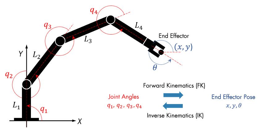
This post addresses the foundational subproblem of forward kinematics: given the joint variables (revolute angles and prismatic displacements), what is the pose of the end-effector relative to the base? Two formulations dominate the literature:
- Denavit-Hartenberg (DH) parameters: each link transformation is encoded by four parameters built on top of a carefully assigned chain of coordinate frames.
- Product of Exponentials (PoE) formula: each joint is treated as a screw, and the forward kinematics is a product of matrix exponentials acting on a fixed home configuration.
We develop both, work the same planar 3R manipulator through each, and compare.
Problem Statement
Consider an open kinematic chain consisting of $n + 1$ links connected by $n$ one-degree-of-freedom joints. We label the links $0, 1, \ldots, n$, where link $0$ is the fixed base and link $n$ carries the end-effector (or “tool”). Joints are numbered $1, \ldots, n$ so that joint $i$ connects link $i - 1$ to link $i$. The motion of each joint is described by a single scalar joint variable $q_i$:
\[q_i = \begin{cases} \theta_i & \text{if joint } i \text{ is revolute}, \\ d_i & \text{if joint } i \text{ is prismatic}. \end{cases}\]Let $\mathbf{q} = (q_1, \ldots, q_n)^\top$ denote the vector of joint variables, and let $T \in SE(3)$ denote the homogeneous transformation that expresses the pose of the end-effector frame with respect to the inertial base frame.
The forward kinematics of an open chain is the map $$ T : \mathbb{R}^n \to SE(3), \qquad \mathbf{q} \;\mapsto\; T(\mathbf{q}) = \begin{bmatrix} R(\mathbf{q}) & \mathbf{p}(\mathbf{q}) \\ \mathbf{0}^\top & 1 \end{bmatrix}, $$ where $R(\mathbf{q}) \in SO(3)$ is the orientation of the end-effector frame in the base frame and $\mathbf{p}(\mathbf{q}) \in \mathbb{R}^3$ is the position of its origin.
The inverse problem, computing $\mathbf{q}$ from a desired $T$, is inverse kinematics, and it will be treated in a separate post. The forward problem is always well-defined and (for serial chains) admits a closed-form expression; the principal task is to systematize its computation.
Links, Joints, and Frames
Before introducing either DH or PoE, we recall some standard modelling assumptions.
Single-DoF Joints
We restrict attention to 1-DoF joints, of which the most common are:
- Revolute (R): allows pure rotation about a fixed axis. The joint variable is the angle $\theta_i$.
- Prismatic (P): allows pure translation along a fixed axis. The joint variable is the displacement $d_i$.
Without loss of generality, any higher-DoF joint can be modelled as a succession of revolute and prismatic joints connected by zero-length links. For instance, a ball-and-socket joint (3 DoF) or a universal joint (2 DoF) reduces to a short chain of revolute joints. Traditionally, in fact, the joints of a manipulator are drawn from just six mechanisms known as the lower pairs, each corresponding to a subgroup of the special Euclidean group $SE(3)$.
$\color{green}{\mathbf{Example\ 1.}}$ The six lower pairs
A kinematic pair is a joint between two links, classified by how their surfaces meet. A lower pair keeps the two links in contact over a surface; a higher pair (gear teeth, a cam and follower, a rolling ball bearing) touches only along a line or at a point. Surface contact permits exactly six kinds of relative motion, and these six lower pairs are the standard joints of manipulators. Each is a connected subgroup of $SE(3)$:
- Revolute (R): rotation about an axis, a zero-pitch screw. The workhorse of robotics.
- Prismatic (P): translation along an axis, an infinite-pitch screw. Just as common.
- Helical (H): rotation coupled to translation along one axis, a screw of finite nonzero pitch.
- Cylindrical (C): independent rotation and translation about a single axis (2 DoF); an R and a P sharing that axis.
- Spherical (S): rotation about a point (3 DoF). A ball-in-socket realizes it passively, but to carry load it is built from three revolute joints whose axes meet at a point, which is how most robot wrists are made.
- Planar: translation and rotation confined to a plane (3 DoF), i.e. motion in $SE(2)$.
Almost every joint on a real manipulator is revolute or prismatic; the rest are assembled from these when needed. This is why modeling a robot with only 1-DoF revolute and prismatic joints costs nothing in generality: a higher-DoF joint is a few of them stacked with zero-length links in between.
A robot manipulator with $n$ such joints therefore has $n + 1$ links (numbered $0, 1, \ldots, n$, where link $0$ is the fixed base) and a configuration space of dimension $n$. The joint variables $(q_1, \ldots, q_n)$ furnish global coordinates on this $n$-dimensional configuration manifold. Joint $i$ is conventionally taken to be fixed with respect to link $i - 1$; equivalently, when joint $i$ is actuated, link $i$ and everything past it in the chain moves. Link $0$ never moves.
Rigid Links
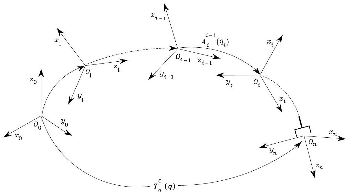
Each link is modeled as a rigid body with a body-fixed frame ${i}$. Composing the transformations between consecutive frames gives the end-effector pose:
\[T_n^0(\mathbf{q}) = T_1^0(q_1)\, T_2^1(q_2) \cdots T_n^{n-1}(q_n).\]Here $T_n^0(\mathbf{q}) \in SE(3)$ is the pose of the end-effector frame ${n}$ relative to the base frame ${0}$: its rotation block $R_n^0$ gives the end-effector’s orientation and its translation block $\mathbf{o}_n^0$ gives the position of its origin, both expressed in ${0}$. The dependence on the joint vector $\mathbf{q} = (q_1, \ldots, q_n)$ enters through the chain product, where each factor
\[T_i^{i-1}(q_i) = \begin{bmatrix} R_i^{i-1} & \mathbf{o}_i^{i-1} \\ \mathbf{0}^\top & 1 \end{bmatrix} \in SE(3)\]depends only on its own joint variable $q_i$ (the geometry of link $i$ itself is fixed) and maps a point from frame ${i}$ to frame ${i-1}$ via $\mathbf{p}_{i-1} = R_i^{i-1}\,\mathbf{p}_i + \mathbf{o}_i^{i-1}$. Then, The chain product acts as
\[T_n^0(\mathbf{q})\, \mathbf{p}_n \;=\; \mathbf{p}_0,\]i.e. it takes a point’s coordinates in the end-effector frame ${n}$ and returns the coordinates of the same geometric point in the base frame ${0}$. The DH and PoE conventions below differ only in how they choose the frames ${i}$ and parameterize each $T_i^{i-1}$.
Denavit-Hartenberg (DH) Parameters
Denavit and Hartenberg introduced their parameterization in 1955 as a compact way to describe serial-chain mechanisms. A generic rigid-body transformation in $SE(3)$ takes six numbers (three for rotation, three for translation), but by constraining how successive link frames are placed, only four per link are needed. An $n$-joint manipulator is therefore fully specified by $4n$ scalars, and a small DH table is enough to encode the entire arm.
Two variants of the convention coexist. The standard (or distal) form [1, 2, 4] attaches frame ${i}$ at the distal end of link $i$ so that $z_i$ is the axis of the next joint, joint $i+1$. The modified (or proximal) form [3] attaches frame ${i}$ at the proximal end so that $z_i$ is the axis of joint $i$ itself. Both produce the same end-effector transform when applied consistently along the chain; we follow the standard form throughout.
Frame Assignment
The single most error-prone step in applying the DH convention is the assignment of link frames. The trick is to constrain the placement of each frame ${i}$ so that its relative pose to the predecessor ${i-1}$ can be encoded by just four numbers. The constraints are the two alignment conditions below, and the standard procedure builds a chain of frames that satisfies them at every joint.
Alignment Conditions
- (DH1) $x_i$ is perpendicular to $z_{i-1}$.
- (DH2) $x_i$ intersects $z_{i-1}$.
Procedure
The standard 6-step algorithm (Spong Section 3.2.2) proceeds as follows.
- Locate joint axes. For each joint $i$, identify the axis of rotation (revolute) or translation (prismatic) and label it $z_{i-1}$. Thus $z_0$ is the axis of joint 1, $z_1$ is the axis of joint 2, and so on.
- Establish the base frame. Choose any point on $z_0$ as the origin $o_0$, then pick $x_0$ and $y_0$ freely to form a right-handed frame.
-
For $i = 1, \ldots, n-1$:
- If $z_i$ and $z_{i-1}$ are not coplanar, the unique common normal between them defines $x_i$, and $o_i$ is the foot of that normal on $z_i$.
- If $z_i$ and $z_{i-1}$ intersect, set $o_i$ at the intersection and choose $x_i$ normal to the plane of $z_{i-1}$ and $z_i$.
- If $z_i$ is parallel to $z_{i-1}$, choose $o_i$ on $z_i$ in any convenient location (often so that $d_i = 0$); pick $x_i$ along the common normal that passes through $o_{i-1}$.
- Choose $y_i$ by the right-hand rule.
- Establish the tool frame ${n}$ at the end-effector. By convention, $z_n$ is the approach direction $\mathbf{a}$, $y_n$ is the sliding direction $\mathbf{s}$, and $x_n = \mathbf{s} \times \mathbf{a}$ is the normal $\mathbf{n}$.
- Read off the DH table $(a_i, \alpha_i, d_i, \theta_i)$ for each link.
Following these steps will always produce a chain that satisfies (DH1) and (DH2) at every joint.
The Four DH Parameters
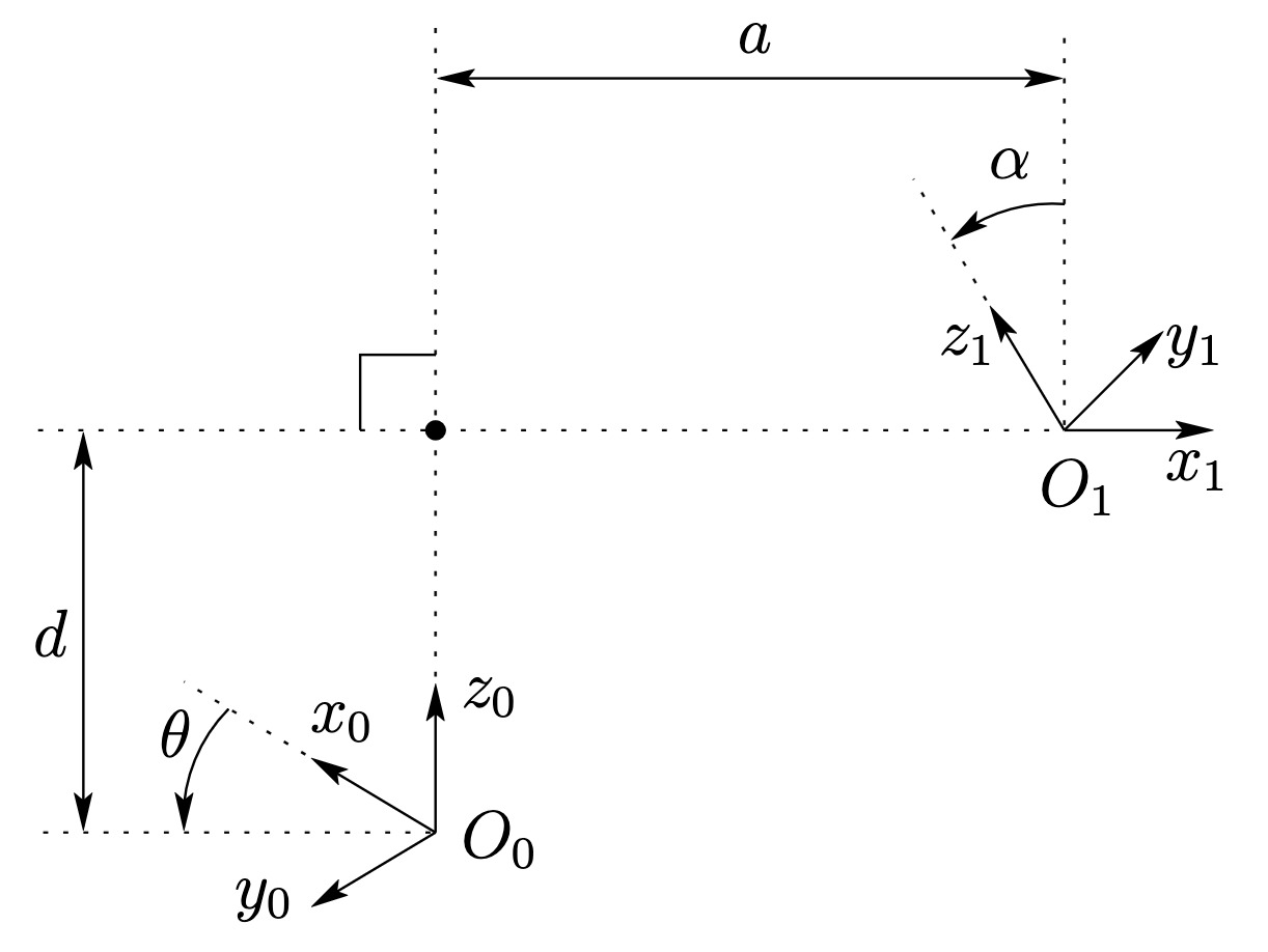
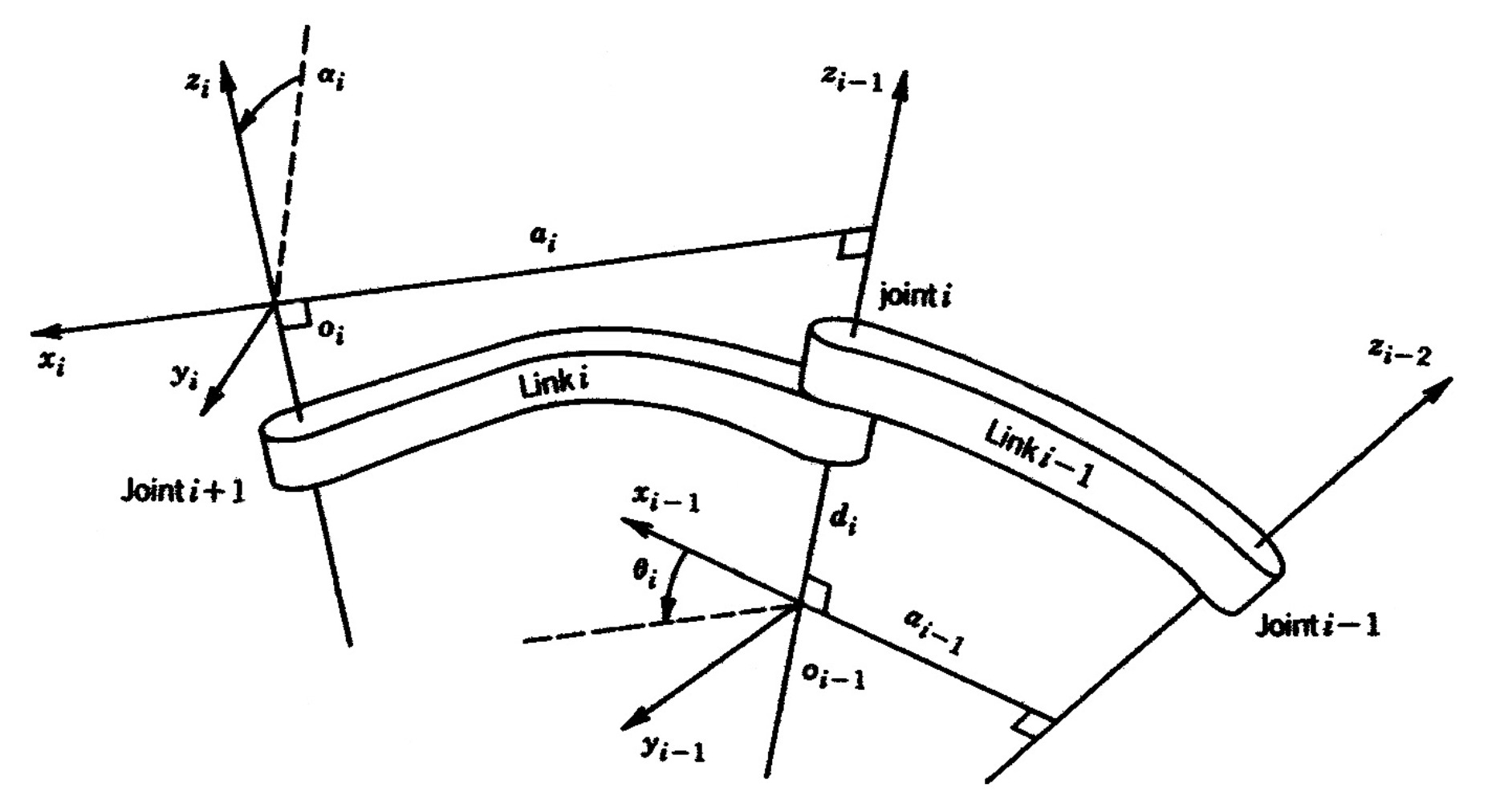
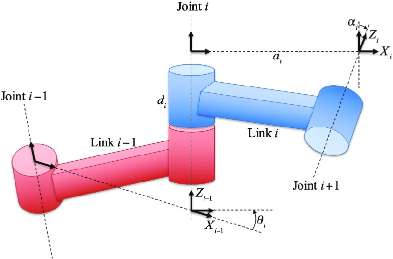
With the frames assigned according to the procedure above, the homogeneous transformation $T_i^{i-1}$ between consecutive frames decomposes into four elementary screws: two rotations and two translations about and along $z_{i-1}$ and $x_i$. The four DH parameters are the magnitudes of these screws, defined geometrically as follows.
- Link length $a_i$: the distance from $z_{i-1}$ to $z_i$ measured along $x_i$.
- Link twist $\alpha_i$: the angle from $z_{i-1}$ to $z_i$ measured about $x_i$ (right-hand rule).
- Link offset $d_i$: the distance from $o_{i-1}$ to the intersection of $x_i$ with $z_{i-1}$, measured along $z_{i-1}$.
- Joint angle $\theta_i$: the angle from $x_{i-1}$ to $x_i$ measured about $z_{i-1}$.
The four parameters split into two pairs with distinct physical meanings:
- Link parameters $(a_i, \alpha_i)$. The link length $a_i$ and link twist $\alpha_i$ describe the common normal between two consecutive joint axes $z_{i-1}$ and $z_i$, the unique line perpendicular to both. Its direction is parallel to $z_{i-1} \times z_i$ and is taken as the body-fixed axis $\hat{x}_i$. The pair $(a_i, \alpha_i)$ records the length of this common normal and the angle by which $z_i$ is rotated relative to $z_{i-1}$ about $\hat{x}_i$. They depend only on the geometry of link $i$ as a manufactured part and are fixed.
- Joint parameters $(d_i, \theta_i)$. The link offset $d_i$ and joint angle $\theta_i$ describe how the next frame is shifted along, and rotated about, the joint axis $z_{i-1}$. One of them is the joint variable (whichever the joint actually moves); the other is a structural constant.
Link Transformation Matrix
Once the four parameters are known, the homogeneous transformation between consecutive frames is the product of four elementary screws,
\[\begin{aligned} A_i &= \mathrm{Rot}_{z, \theta_i}\,\mathrm{Trans}_{z, d_i}\,\mathrm{Trans}_{x, a_i}\,\mathrm{Rot}_{x, \alpha_i} \\[4pt] &= \begin{bmatrix} \cos\theta_i & -\sin\theta_i & 0 & 0 \\ \sin\theta_i & \cos\theta_i & 0 & 0 \\ 0 & 0 & 1 & 0 \\ 0 & 0 & 0 & 1 \end{bmatrix} \begin{bmatrix} 1 & 0 & 0 & 0 \\ 0 & 1 & 0 & 0 \\ 0 & 0 & 1 & d_i \\ 0 & 0 & 0 & 1 \end{bmatrix} \begin{bmatrix} 1 & 0 & 0 & a_i \\ 0 & 1 & 0 & 0 \\ 0 & 0 & 1 & 0 \\ 0 & 0 & 0 & 1 \end{bmatrix} \begin{bmatrix} 1 & 0 & 0 & 0 \\ 0 & \cos\alpha_i & -\sin\alpha_i & 0 \\ 0 & \sin\alpha_i & \cos\alpha_i & 0 \\ 0 & 0 & 0 & 1 \end{bmatrix} \\[4pt] &= \begin{bmatrix} \cos\theta_i & -\sin\theta_i \cos\alpha_i & \sin\theta_i \sin\alpha_i & a_i \cos\theta_i \\ \sin\theta_i & \cos\theta_i \cos\alpha_i & -\cos\theta_i \sin\alpha_i & a_i \sin\theta_i \\ 0 & \sin\alpha_i & \cos\alpha_i & d_i \\ 0 & 0 & 0 & 1 \end{bmatrix}. \end{aligned}\]We denote this transformation between consecutive frames by $T_i^{i-1}$:
\[T_i^{i-1} \;\equiv\; A_i(q_i).\]The forward kinematics of an $n$-joint serial chain is then
\[T_n^0(\mathbf{q}) \;=\; T_1^0(q_1)\, T_2^1(q_2) \cdots T_n^{n-1}(q_n) \;=\; \prod_{i=1}^{n} A_i(q_i).\]$\color{green}{\mathbf{Example\ 2.}}$ Planar 3R manipulator via DH
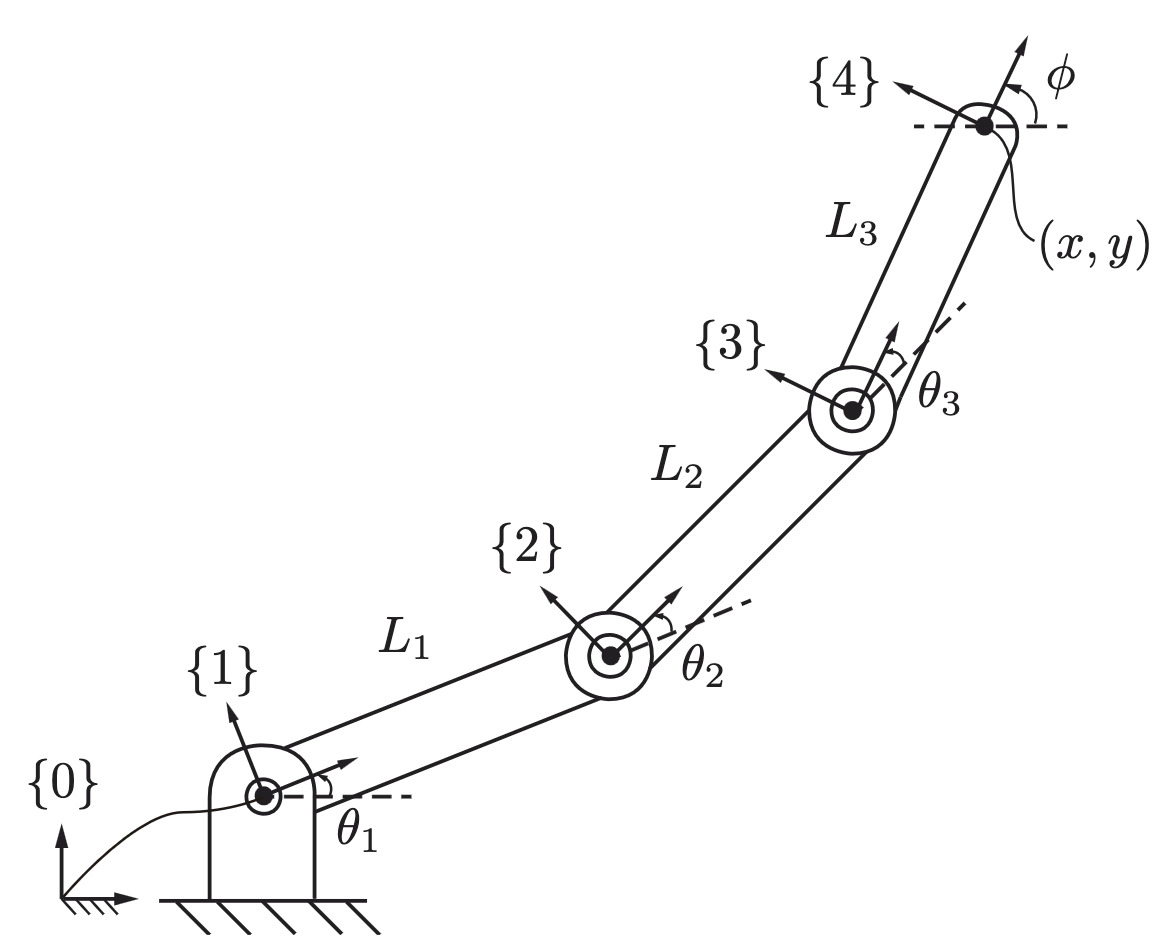
We apply the DH algorithm to a planar three-revolute (3R) manipulator with link lengths $L_1, L_2, L_3$. All joint axes are parallel and out of the page, so we expect every $\alpha_i = 0$ and every $d_i = 0$.
Frame Assignment.
- $z_0, z_1, z_2$ all point out of the page (joint rotation axes).
- The base origin $o_0$ is at joint 1; $x_0$ points along the first link in the home configuration.
- For each subsequent frame we place $o_i$ at joint $i+1$ and align $x_i$ with link $i$ in the home configuration.
- The tool frame ${3}$ sits at the tip of link 3.
DH Table.
| Link $i$ | $a_i$ | $\alpha_i$ | $d_i$ | $\theta_i$ |
|---|---|---|---|---|
| 1 | $L_1$ | 0 | 0 | $\theta_1^\star$ |
| 2 | $L_2$ | 0 | 0 | $\theta_2^\star$ |
| 3 | $L_3$ | 0 | 0 | $\theta_3^\star$ |
(The starred quantities are the joint variables.)
Link Transformations. The three DH transformations are
\[T_1^0 = \begin{bmatrix} \cos\theta_1 & -\sin\theta_1 & 0 & L_1 \cos\theta_1 \\ \sin\theta_1 & \cos\theta_1 & 0 & L_1 \sin\theta_1 \\ 0 & 0 & 1 & 0 \\ 0 & 0 & 0 & 1 \end{bmatrix}, \quad T_2^1 = \begin{bmatrix} \cos\theta_2 & -\sin\theta_2 & 0 & L_2 \cos\theta_2 \\ \sin\theta_2 & \cos\theta_2 & 0 & L_2 \sin\theta_2 \\ 0 & 0 & 1 & 0 \\ 0 & 0 & 0 & 1 \end{bmatrix},\] \[T_3^2 = \begin{bmatrix} \cos\theta_3 & -\sin\theta_3 & 0 & L_3 \cos\theta_3 \\ \sin\theta_3 & \cos\theta_3 & 0 & L_3 \sin\theta_3 \\ 0 & 0 & 1 & 0 \\ 0 & 0 & 0 & 1 \end{bmatrix}.\]Step-by-Step Chain Product. The cumulative transform from base to frame ${2}$ is
\[T_2^0 = T_1^0 T_2^1 = \begin{bmatrix} \cos(\theta_1+\theta_2) & -\sin(\theta_1+\theta_2) & 0 & L_1 \cos\theta_1 + L_2 \cos(\theta_1+\theta_2) \\ \sin(\theta_1+\theta_2) & \cos(\theta_1+\theta_2) & 0 & L_1 \sin\theta_1 + L_2 \sin(\theta_1+\theta_2) \\ 0 & 0 & 1 & 0 \\ 0 & 0 & 0 & 1 \end{bmatrix},\]which already exposes the planar nature of the manipulator: orientations of all intermediate frames are pure $z$-axis rotations whose angles add, and positions are the obvious sum of in-plane link-length vectors.
End-Effector Pose. The chain product is
\[T_3^0 = T_1^0 T_2^1 T_3^2 = \begin{bmatrix} \cos(\theta_1+\theta_2+\theta_3) & -\sin(\theta_1+\theta_2+\theta_3) & 0 & L_1 \cos\theta_1 + L_2 \cos(\theta_1+\theta_2) + L_3 \cos(\theta_1+\theta_2+\theta_3) \\ \sin(\theta_1+\theta_2+\theta_3) & \cos(\theta_1+\theta_2+\theta_3) & 0 & L_1 \sin\theta_1 + L_2 \sin(\theta_1+\theta_2) + L_3 \sin(\theta_1+\theta_2+\theta_3) \\ 0 & 0 & 1 & 0 \\ 0 & 0 & 0 & 1 \end{bmatrix}.\]Reading off the position of the end-effector,
\[x = L_1 \cos\theta_1 + L_2 \cos(\theta_1 + \theta_2) + L_3 \cos(\theta_1 + \theta_2 + \theta_3),\] \[y = L_1 \sin\theta_1 + L_2 \sin(\theta_1 + \theta_2) + L_3 \sin(\theta_1 + \theta_2 + \theta_3),\] \[\phi = \theta_1 + \theta_2 + \theta_3,\]which matches the elementary trigonometric derivation given by Lynch and Park (equations 4.1-4.3).
$\color{green}{\mathbf{Example\ 3.}}$ Spherical (RRP) arm
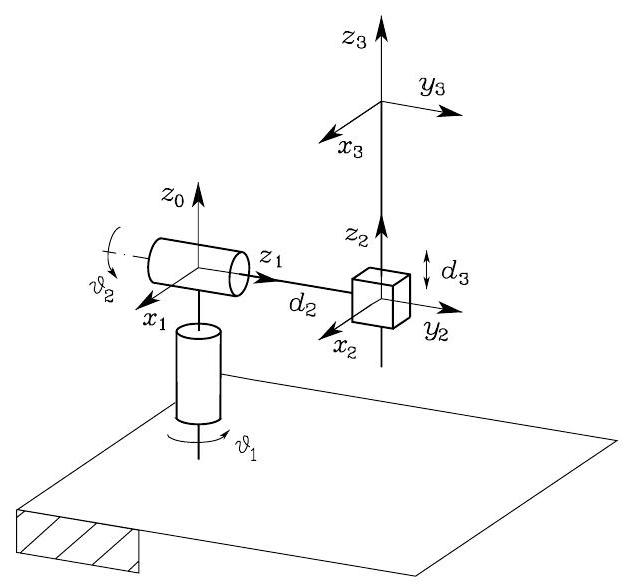
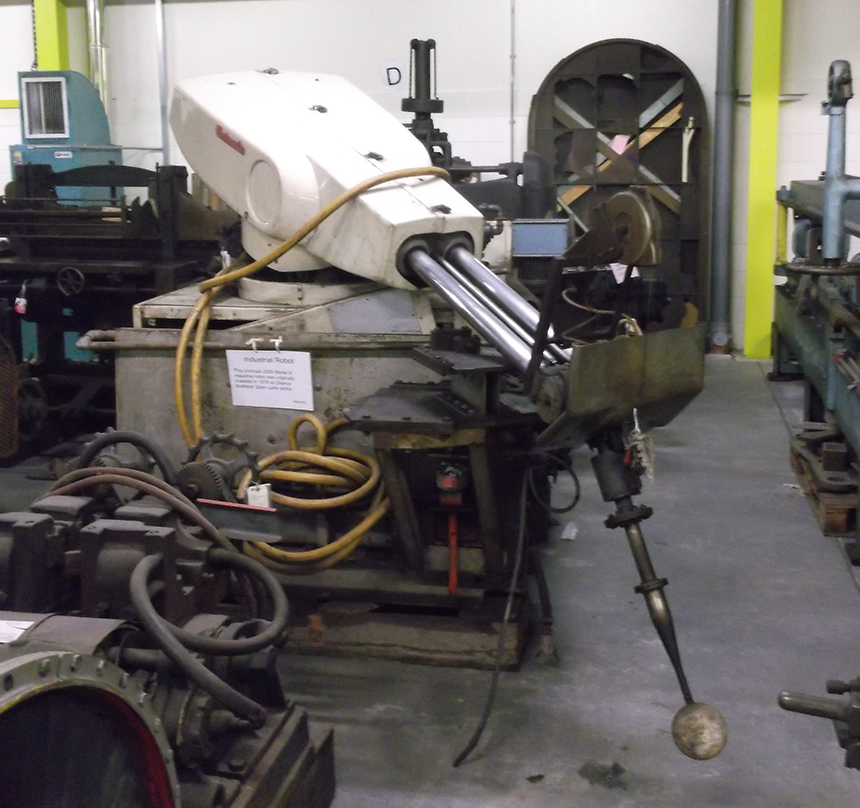
A spherical arm positions the end-effector in spherical coordinates: azimuth $\theta_1$ rotates about a vertical base axis, polar angle $\theta_2$ swings the boom in elevation, and prismatic extension $d_3$ moves it radially. It is the configuration of cranes and many early industrial pick-and-place arms.
DH Table.
| Link $i$ | $a_i$ | $\alpha_i$ | $d_i$ | $\theta_i$ |
|---|---|---|---|---|
| 1 | 0 | $-\pi/2$ | 0 | $\theta_1^\star$ |
| 2 | 0 | $\pi/2$ | $d_2$ | $\theta_2^\star$ |
| 3 | 0 | 0 | $d_3^\star$ | 0 |
End-Effector Pose.
\[T_3^0 = \begin{bmatrix} \cos\theta_1\cos\theta_2 & -\sin\theta_1 & \cos\theta_1\sin\theta_2 & \cos\theta_1\sin\theta_2\, d_3 - \sin\theta_1\, d_2 \\ \sin\theta_1\cos\theta_2 & \cos\theta_1 & \sin\theta_1\sin\theta_2 & \sin\theta_1\sin\theta_2\, d_3 + \cos\theta_1\, d_2 \\ -\sin\theta_2 & 0 & \cos\theta_2 & \cos\theta_2\, d_3 \\ 0 & 0 & 0 & 1 \end{bmatrix}.\]$\color{green}{\mathbf{Example\ 4.}}$ Anthropomorphic (3R) arm
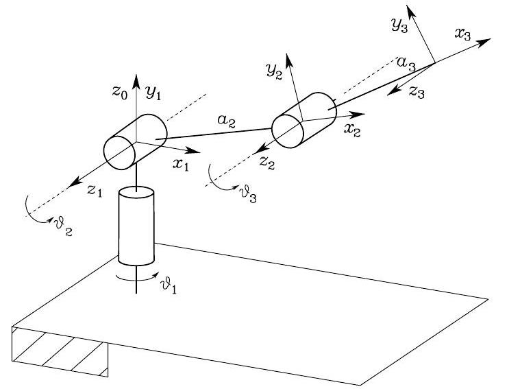
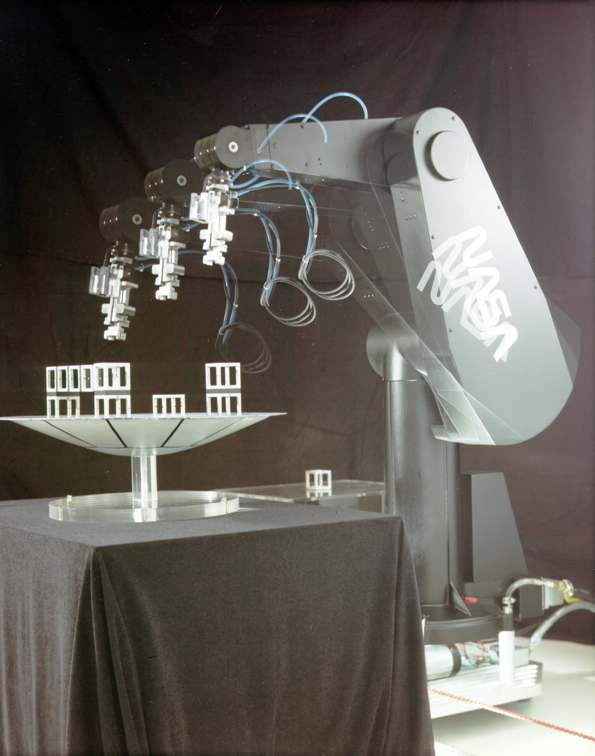
An anthropomorphic arm has three revolute joints: $\theta_1$ rotates about a vertical “shoulder” axis, and $\theta_2, \theta_3$ swing the upper arm and forearm in the resulting vertical plane. This is the kinematic core of most articulated industrial robots.
DH Table.
| Link $i$ | $a_i$ | $\alpha_i$ | $d_i$ | $\theta_i$ |
|---|---|---|---|---|
| 1 | 0 | $\pi/2$ | 0 | $\theta_1^\star$ |
| 2 | $a_2$ | 0 | 0 | $\theta_2^\star$ |
| 3 | $a_3$ | 0 | 0 | $\theta_3^\star$ |
End-Effector Pose.
\[T_3^0 = \begin{bmatrix} \cos\theta_1 \cos(\theta_2+\theta_3) & -\cos\theta_1 \sin(\theta_2+\theta_3) & \sin\theta_1 & \cos\theta_1 \big( a_2 \cos\theta_2 + a_3 \cos(\theta_2+\theta_3) \big) \\ \sin\theta_1 \cos(\theta_2+\theta_3) & -\sin\theta_1 \sin(\theta_2+\theta_3) & -\cos\theta_1 & \sin\theta_1 \big( a_2 \cos\theta_2 + a_3 \cos(\theta_2+\theta_3) \big) \\ \sin(\theta_2+\theta_3) & \cos(\theta_2+\theta_3) & 0 & a_2 \sin\theta_2 + a_3 \sin(\theta_2+\theta_3) \\ 0 & 0 & 0 & 1 \end{bmatrix}.\]$\color{green}{\mathbf{Example\ 5.}}$ Spherical wrist (3R)
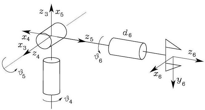
A spherical wrist consists of three revolute joints whose axes meet at a single point, giving the end-effector arbitrary orientation about that point. It is the standard wrist subassembly attached after a 3-DoF positioning arm to give a full 6-DoF manipulator. The joints are indexed $4, 5, 6$ (continuing the chain from a 3-DoF arm), and the wrist center is the origin of frame ${3}$.
DH Table.
| Link $i$ | $a_i$ | $\alpha_i$ | $d_i$ | $\theta_i$ |
|---|---|---|---|---|
| 4 | 0 | $-\pi/2$ | 0 | $\theta_4^\star$ |
| 5 | 0 | $\pi/2$ | 0 | $\theta_5^\star$ |
| 6 | 0 | 0 | $d_6$ | $\theta_6^\star$ |
Wrist Transformation.
\[T_6^3 = \begin{bmatrix} \cos\theta_4 \cos\theta_5 \cos\theta_6 - \sin\theta_4 \sin\theta_6 & -\cos\theta_4 \cos\theta_5 \sin\theta_6 - \sin\theta_4 \cos\theta_6 & \cos\theta_4 \sin\theta_5 & \cos\theta_4 \sin\theta_5\, d_6 \\ \sin\theta_4 \cos\theta_5 \cos\theta_6 + \cos\theta_4 \sin\theta_6 & -\sin\theta_4 \cos\theta_5 \sin\theta_6 + \cos\theta_4 \cos\theta_6 & \sin\theta_4 \sin\theta_5 & \sin\theta_4 \sin\theta_5\, d_6 \\ -\sin\theta_5 \cos\theta_6 & \sin\theta_5 \sin\theta_6 & \cos\theta_5 & \cos\theta_5\, d_6 \\ 0 & 0 & 0 & 1 \end{bmatrix}.\]The rotation block is precisely the ZYZ Euler-angle parameterization of orientation; the spherical wrist therefore has the same singularity (at $\theta_5 = 0, \pi$) as the ZYZ chart of $SO(3)$.
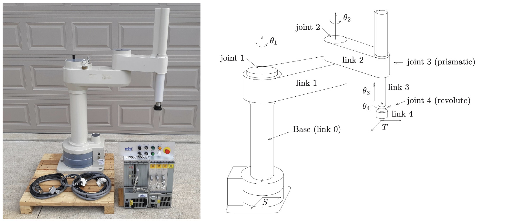
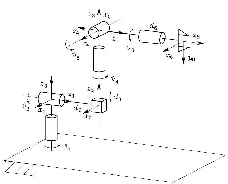
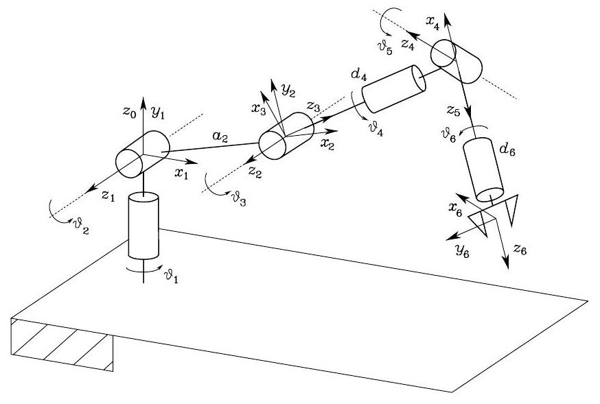
$\color{green}{\mathbf{Example\ 6.}}$ Stanford manipulator (RRP + spherical wrist)
.jpg)
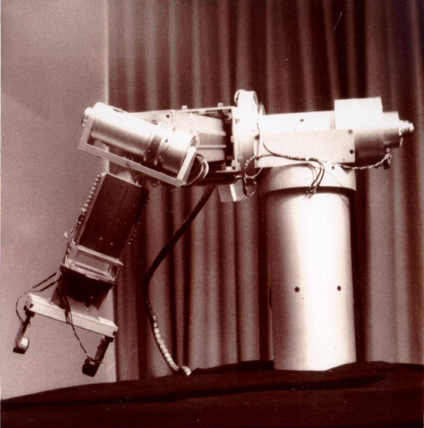
The classic Stanford manipulator (Victor Scheinman, 1969) concatenates a spherical (RRP) arm with a spherical wrist to give a 6-DoF arm whose positioning (joints 1–3) and orientation (joints 4–6) subchains decouple at the wrist center. The DH table is the concatenation of Examples 3 and 5.
For brevity in this and the next example we use the shorthand $c_i \equiv \cos\theta_i$, $s_i \equiv \sin\theta_i$, with compound-angle abbreviations such as $c_{23} \equiv \cos(\theta_2 + \theta_3)$.
End-Effector Position.
The translation part of the chain product $T_6^0 = T_1^0 T_2^1 \cdots T_6^5$ is
\[\mathbf{p}_6^0 = \begin{bmatrix} c_1 s_2 d_3 - s_1 d_2 + \big( c_1 ( c_2 c_4 s_5 + s_2 c_5 ) - s_1 s_4 s_5 \big) d_6 \\ s_1 s_2 d_3 + c_1 d_2 + \big( s_1 ( c_2 c_4 s_5 + s_2 c_5 ) + c_1 s_4 s_5 \big) d_6 \\ c_2 d_3 + ( -s_2 c_4 s_5 + c_2 c_5 ) d_6 \end{bmatrix}.\]The first terms in each row come from the spherical-arm sub-chain (positioning the wrist center), and the $d_6$-multiplied terms are the offset from the wrist center to the tool tip along the final wrist axis.
$\color{green}{\mathbf{Example\ 7.}}$ Anthropomorphic arm with spherical wrist (6R)
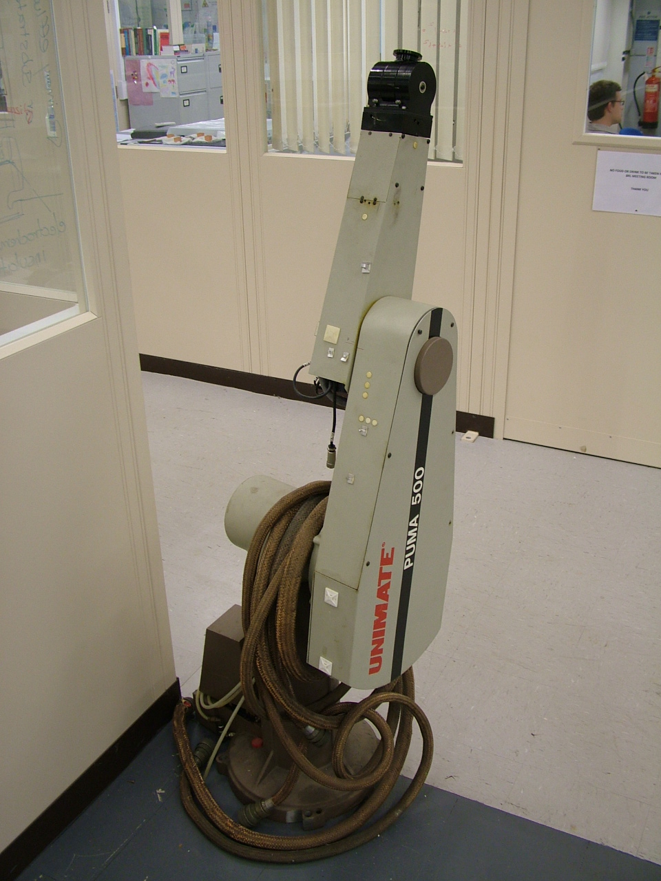
This is the canonical 6-revolute industrial arm — the geometry of the PUMA 560, KUKA KR series, and many modern collaborative manipulators. The base is an anthropomorphic 3R chain (Example 4), and the wrist is a 3R spherical wrist (Example 5).
DH Table.
| Link $i$ | $a_i$ | $\alpha_i$ | $d_i$ | $\theta_i$ |
|---|---|---|---|---|
| 1 | 0 | $\pi/2$ | 0 | $\theta_1^\star$ |
| 2 | $a_2$ | 0 | 0 | $\theta_2^\star$ |
| 3 | 0 | $\pi/2$ | 0 | $\theta_3^\star$ |
| 4 | 0 | $-\pi/2$ | $d_4$ | $\theta_4^\star$ |
| 5 | 0 | $\pi/2$ | 0 | $\theta_5^\star$ |
| 6 | 0 | 0 | $d_6$ | $\theta_6^\star$ |
End-Effector Position.
Using the same shorthand as Example 6 (with $c_{23} \equiv \cos(\theta_2+\theta_3)$, $s_{23} \equiv \sin(\theta_2+\theta_3)$),
\[\mathbf{p}_6^0 = \begin{bmatrix} a_2 c_1 c_2 + d_4 c_1 s_{23} + d_6 \big( c_1 ( c_{23} c_4 s_5 + s_{23} c_5 ) + s_1 s_4 s_5 \big) \\ a_2 s_1 c_2 + d_4 s_1 s_{23} + d_6 \big( s_1 ( c_{23} c_4 s_5 + s_{23} c_5 ) - c_1 s_4 s_5 \big) \\ a_2 s_2 - d_4 c_{23} + d_6 \big( s_{23} c_4 s_5 - c_{23} c_5 \big) \end{bmatrix}.\]Setting $d_4 = d_6 = 0$ recovers the wrist-center position $a_2 ( c_1 c_2,\; s_1 c_2,\; s_2 )^\top$ of the pure anthropomorphic arm of Example 4.
Existence and Uniqueness
The alignment conditions (DH1) and (DH2) are precisely the constraints that reduce a generic six-parameter rigid-body transformation to a four-parameter one, with no remaining ambiguity. The next theorem formalizes this.
Under the alignment conditions (DH1) and (DH2), four parameters suffice to specify the link transformation, and they are uniquely determined: there exist unique numbers $(\theta_i, d_i, a_i, \alpha_i) \in \mathbb{R}^4$ such that the link transformation factors as $$ T_i^{i-1} \;=\; \mathrm{Rot}_{z, \theta_i}\, \mathrm{Trans}_{z, d_i}\, \mathrm{Trans}_{x, a_i}\, \mathrm{Rot}_{x, \alpha_i}. $$
$\color{red}{\mathbf{Proof.}}$
A general element of $SE(3)$ has six independent parameters: three for $R_i^{i-1} \in SO(3)$ and three for the translation $\mathbf{o}_i^{i-1} \in \mathbb{R}^3$. We show existence by explicit construction, i.e. that (DH1) and (DH2) each remove one parameter, leaving four, and then verify uniqueness.
Existence. Write $R_i^{i-1} = [r_{jk}]$. Its first column equals \(\hat{x}_i\) expressed in frame ${i-1}$, while \(\hat{z}_{i-1}\) in the same frame is \(\hat{e}_3 = (0, 0, 1)^\top\). Condition (DH1) yields
\[0 \;=\; \hat{x}_i \cdot \hat{z}_{i-1} \;=\; r_{31}.\]Combined with $R^\top R = I$, the first column lies in the $xy$-plane and the third row lies in the $yz$-plane, so they admit parameterizations
\[\text{col}_1(R) \;=\; \begin{bmatrix}\cos\theta_i\\\\ \sin\theta_i\\\\ 0\end{bmatrix}, \qquad \text{row}_3(R) \;=\; \begin{bmatrix}0 & \sin\alpha_i & \cos\alpha_i\end{bmatrix},\]for some angles $\theta_i, \alpha_i$. The remaining four entries are then determined by orthonormality, giving
\[R_i^{i-1} \;=\; \begin{bmatrix} \cos\theta_i & -\sin\theta_i \cos\alpha_i & \sin\theta_i \sin\alpha_i \\\\ \sin\theta_i & \cos\theta_i \cos\alpha_i & -\cos\theta_i \sin\alpha_i \\\\ 0 & \sin\alpha_i & \cos\alpha_i \end{bmatrix}.\]For the translation, condition (DH2) requires the line of \(\hat{x}_i\) to intersect the line of \(\hat{z}_{i-1}\), so the origin $o_i$ can be reached from \(o_{i-1}\) by a displacement along \(\hat{z}_{i-1}\) followed by a displacement along \(\hat{x}_i\):
\[\mathbf{o}_i^{i-1} \;=\; d_i\, \hat{z}_{i-1} + a_i\, \hat{x}_i \;=\; \begin{bmatrix} a_i \cos\theta_i \\\\ a_i \sin\theta_i \\\\ d_i \end{bmatrix}.\]Combining the rotation and translation, $T_i^{i-1}$ factors as the four-screw product with parameters $(\theta_i, d_i, a_i, \alpha_i)$, so four parameters suffice. The two screws absent from the factorization, \(\mathrm{Rot}_y\) and \(\mathrm{Trans}_y\), are precisely the degrees of freedom that the alignment rules eliminate: (DH1) forbids \(\mathrm{Rot}_y\) since any rotation about \(\hat{y}_{i-1}\) would tilt \(\hat{x}_i\) out of the $xy$-plane and violate $r_{31} = 0$, while (DH2) forbids \(\mathrm{Trans}_y\) since any displacement along \(\hat{y}_{i-1}\) would push $o_i$ off the plane spanned by \(\hat{z}_{i-1}\) and \(\hat{x}_i\).
Uniqueness. Given the entries of $T_i^{i-1}$, the four parameters can be recovered as single-valued functions of those entries:
\[\theta_i \;=\; \mathrm{atan2}(r_{21},\, r_{11}), \qquad \alpha_i \;=\; \mathrm{atan2}(r_{32},\, r_{33}),\] \[a_i \;=\; o_x \cos\theta_i + o_y \sin\theta_i, \qquad d_i \;=\; o_z,\]where $(o_x, o_y, o_z)^\top = \mathbf{o}_i^{i-1}$. The angles are determined modulo $2\pi$; with that convention fixed, the tuple $(\theta_i, d_i, a_i, \alpha_i) \in \mathbb{R}^4$ is unique. $\blacksquare$
A natural follow-up question is whether the count can be reduced even further: could a cleverer set of frame-assignment rules encode each link transformation with three numbers instead of four? Denavit and Hartenberg [4] themselves showed that the answer is no — four is the minimum number of parameters needed to describe the relative pose of two consecutive link frames satisfying (DH1) and (DH2). The DH parameterization is therefore not only sufficient and unique, but also minimal: no convention with fewer parameters per link can capture every admissible relative pose.
Drawbacks
Despite its dominance in textbooks, the DH parameterization has several practical drawbacks that have driven the community toward alternatives.
1. Non-uniqueness of the frame assignment
The Theorem guarantees that the four parameters are unique given a chain of frames satisfying (DH1)–(DH2). The frame assignment itself is not: the placement of $o_i$ along $z_i$, the sign of $z_i$, and the direction of $x_i$ when consecutive joint axes are coplanar all admit multiple valid choices.
2. Hidden coupling between link geometry and joint motion
Inspect the DH link matrix entry by entry,
\[A_i(\theta_i) \;=\; \begin{bmatrix} \cos\theta_i & -\sin\theta_i \cos\alpha_i & \sin\theta_i \sin\alpha_i & a_i \cos\theta_i \\ \sin\theta_i & \cos\theta_i \cos\alpha_i & -\cos\theta_i \sin\alpha_i & a_i \sin\theta_i \\ 0 & \sin\alpha_i & \cos\alpha_i & d_i \\ 0 & 0 & 0 & 1 \end{bmatrix}.\]The joint variable $\theta_i$ (the only quantity that changes as the robot moves, for a revolute joint) is multiplied by triagonal functions of $\alpha_i$ in every off-diagonal entry, and the translation column carries $a_i$. Structural ($\alpha_i, a_i$) and motion ($\theta_i$) factors are interleaved everywhere.
Differentiating in $\theta_i$ gives
\[\frac{\partial A_i}{\partial \theta_i} \;=\; \begin{bmatrix} -\sin\theta_i & -\cos\theta_i \cos\alpha_i & \cos\theta_i \sin\alpha_i & -a_i \sin\theta_i \\ \cos\theta_i & -\sin\theta_i \cos\alpha_i & \sin\theta_i \sin\alpha_i & a_i \cos\theta_i \\ 0 & 0 & 0 & 0 \\ 0 & 0 & 0 & 0 \end{bmatrix},\]still riddled with $\cos\alpha_i, \sin\alpha_i, a_i$. The “joint motion” derivative is heavy with structural constants.
PoE has the opposite structure: $A_i(\theta_i) = e^{[\mathcal{S}_i]\, \theta_i}$. All structural information (joint type, axis direction, axis location, pitch) lives in $\mathcal{S}_i$, with $\theta_i$ as its sole multiplier. Differentiation slides $[\mathcal{S}_i]$ out cleanly:
\[\frac{\partial}{\partial \theta_i}\, e^{[\mathcal{S}_i]\, \theta_i} \;=\; [\mathcal{S}_i]\, e^{[\mathcal{S}_i]\, \theta_i}.\]This is what makes PoE Jacobian columns simple: each column is the joint’s screw axis (pure geometry) transported by the rest of the chain (pure motion), with no structural-motion cross-terms.
Product of Exponentials (PoE) Formula
The Product of Exponentials (PoE) formula is an alternative to the Denavit–Hartenberg parameterization for describing the forward kinematics of a spatial kinematic chain. While DH uses the minimal number of parameters per link, PoE has a number of advantages:
- Uniform treatment of revolute and prismatic joints. Each joint is encoded by a single 6-vector screw axis $\mathcal{S}_i$, regardless of joint type.
- Only two reference frames. A fixed base frame and a body-fixed end-effector frame at the home configuration suffice; no intermediate link frames need to be assigned.
- Direct geometric interpretation. Each $\mathcal{S}_i$ is the joint's screw axis at the home configuration, expressed in the base frame; its physical meaning is immediately visible.
The formula admits two equivalent forms: the space form, in which each screw axis is expressed in the inertial base frame, and the body form, in which each screw axis is expressed in the end-effector frame.
Space Form
The PoE formulation rests on a single geometric insight: a one-DoF joint generates a screw motion of the rigid body it carries, and a screw motion in $SE(3)$ is the matrix exponential of a twist (an element of the Lie algebra $\mathfrak{se}(3)$).
Recap: Twists and Screw Axes
From the previous post, recall that a unit twist or screw axis is a 6-vector $\mathcal{S} = (\boldsymbol{\omega}, \mathbf{v}) \in \mathbb{R}^6$ that admits the matrix form
\[[\mathcal{S}] = \begin{bmatrix} [\boldsymbol{\omega}] & \mathbf{v} \\ \mathbf{0}^\top & 0 \end{bmatrix} \in \mathfrak{se}(3),\]where $[\boldsymbol{\omega}] \in \mathfrak{so}(3)$ is the $3 \times 3$ skew-symmetric form of $\boldsymbol{\omega}$. For a revolute joint of axis direction $\hat{\boldsymbol{\omega}}$ passing through a point $\mathbf{q}$ (in the fixed base frame),
\[\boldsymbol{\omega} = \hat{\boldsymbol{\omega}}, \qquad \mathbf{v} = -\hat{\boldsymbol{\omega}} \times \mathbf{q}.\]For a prismatic joint of direction $\hat{\mathbf{v}}$,
\[\boldsymbol{\omega} = \mathbf{0}, \qquad \mathbf{v} = \hat{\mathbf{v}}.\]The matrix exponential $e^{[\mathcal{S}] \theta} \in SE(3)$ rigidly displaces a body by an amount $\theta$ along the screw $\mathcal{S}$.
Derivation of the Space-Form PoE
Choose a fixed base frame \(\{s\}\) and let $M \in SE(3)$ denote the home configuration of the end-effector frame \(\{b\}\) relative to \(\{s\}\) (the value of the end-effector pose when all joint variables are zero). Let $\mathcal{S}_i$ be the screw axis of joint $i$, expressed in \(\{s\}\) when the chain is in its home configuration.
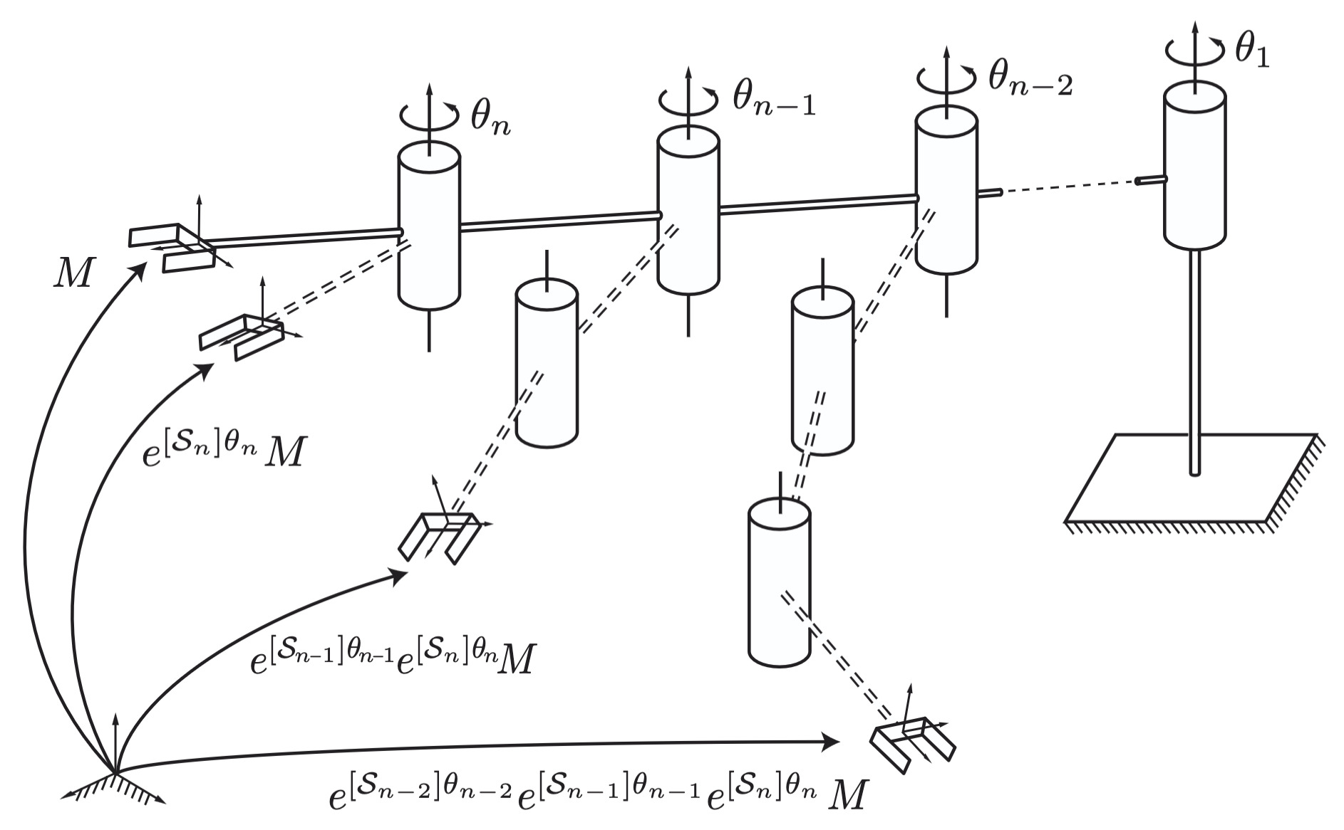
First, if only joint $n$ moves,
\[T = e^{[\mathcal{S}_n] \theta_n} M.\]If we now also let joint $n - 1$ move while keeping the rest fixed, the rigid sub-chain consisting of link $n - 1$ and link $n$ is displaced by a screw motion about $\mathcal{S}_{n-1}$:
\[T = e^{[\mathcal{S}_{n-1}] \theta_{n-1}}\, e^{[\mathcal{S}_n] \theta_n}\, M.\]Continuing recursively for all $n$ joints yields the space form of the PoE.
For an $n$-joint open chain with screw axes $\mathcal{S}_1, \ldots, \mathcal{S}_n$ expressed in the fixed base frame at the home configuration $M \in SE(3)$, $$ T(\boldsymbol{\theta}) \;=\; e^{[\mathcal{S}_1] \theta_1}\, e^{[\mathcal{S}_2] \theta_2} \cdots e^{[\mathcal{S}_n] \theta_n}\, M. $$
To use the formula one needs only three ingredients:
- The home configuration $M$,
- The list of screw axes $\mathcal{S}_1, \ldots, \mathcal{S}_n$ in the fixed frame at the home configuration,
- The joint values $\boldsymbol{\theta} = (\theta_1, \ldots, \theta_n)$.
No intermediate link frames are required.
Body Form
There is a dual formulation in which the screw axes are expressed in the end-effector (body) frame at the home configuration. The key tool is the adjoint map, which transforms twists between frames. For $T = \begin{bmatrix} R & \mathbf{p} ; \mathbf{0}^\top & 1 \end{bmatrix} \in SE(3)$,
\[\mathrm{Ad}_T = \begin{bmatrix} R & 0 \\ [\mathbf{p}] R & R \end{bmatrix} \in \mathbb{R}^{6 \times 6},\]acting on a twist $\mathcal{V} = (\boldsymbol{\omega}, \mathbf{v}) \in \mathbb{R}^6$. The adjoint encodes how a screw axis seen in one frame appears in another. Using the matrix identity $e^{M^{-1} P M} = M^{-1} e^P M$ for any $P \in \mathfrak{se}(3)$ and any $M \in SE(3)$ (it can be derived easily with matrix exponential formula), one can push each $M$ to the left:
\[\begin{aligned} T(\boldsymbol{\theta}) &= e^{[\mathcal{S}_1] \theta_1} \cdots e^{[\mathcal{S}_n] \theta_n}\, M \\ &= M e^{M^{-1} [\mathcal{S}_1] M \theta_1} \cdots e^{M^{-1} [\mathcal{S}_n] M \theta_n} \\ &= M e^{[\mathcal{B}_1] \theta_1}\, e^{[\mathcal{B}_2] \theta_2} \cdots e^{[\mathcal{B}_n] \theta_n}, \end{aligned}\]where each body-frame screw axis $\mathcal{B}_i$ is related to its space-frame counterpart by the adjoint map
\[\mathcal{B}_i \;=\; \mathrm{Ad}_{M^{-1}}\, \mathcal{S}_i, \qquad i = 1, \ldots, n.\]For the same open chain with body-frame screw axes $\mathcal{B}_i = \mathrm{Ad}_{M^{-1}} \mathcal{S}_i$, $$ T(\boldsymbol{\theta}) \;=\; M\, e^{[\mathcal{B}_1] \theta_1}\, e^{[\mathcal{B}_2] \theta_2} \cdots e^{[\mathcal{B}_n] \theta_n}. $$
The interpretation differs: in the space form, $M$ is transformed first by the last joint (nearest the end-effector) and the action progresses inward; in the body form, $M$ is transformed first by the first joint (nearest the base) and progresses outward. The two are algebraically equivalent.
$\color{green}{\mathbf{Example\ 8.}}$ Universal Robots' UR5 6R arm via PoE
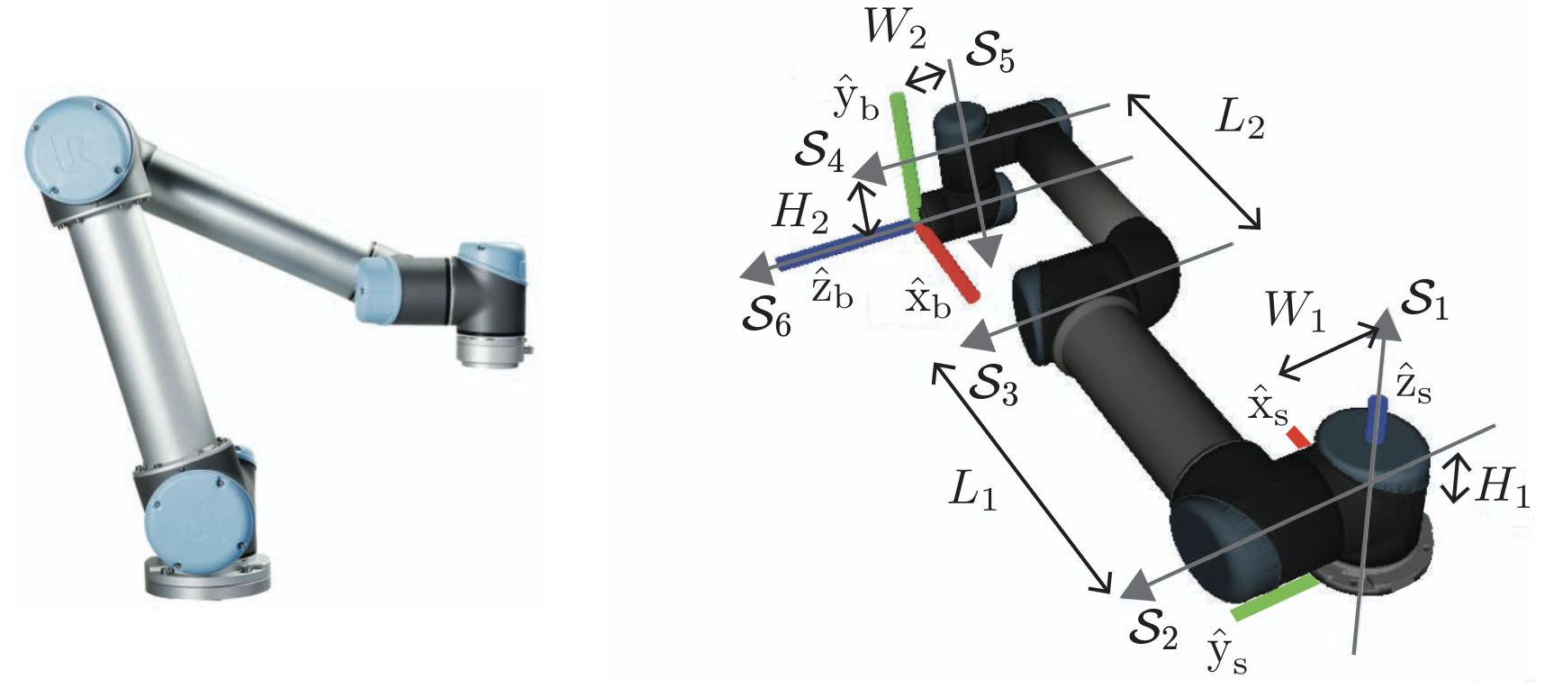
The UR5 has six revolute joints, and at the zero pose shown above every joint axis aligns with $\hat{x}_s$, $\hat{y}_s$, or $\pm\hat{z}_s$. PoE needs only two ingredients: the home configuration $M$ and one screw $\mathcal{S}_i$ per joint.
Home configuration. At the zero pose, the end-effector frame ${b}$ has origin
\[\mathbf{p}_{\text{home}} \;=\; (L_1 + L_2,\; W_1 + W_2,\; H_1 - H_2),\]and its axes, read off the right panel, satisfy $(\hat{x}_b,\,\hat{y}_b,\,\hat{z}_b) = (-\hat{x}_s,\,\hat{z}_s,\,\hat{y}_s)$, giving
\[M \;=\; \begin{bmatrix} -1 & 0 & 0 & L_1 + L_2 \\ 0 & 0 & 1 & W_1 + W_2 \\ 0 & 1 & 0 & H_1 - H_2 \\ 0 & 0 & 0 & 1 \end{bmatrix}.\]Screw axes in the fixed frame. For each joint, pick any point $\mathbf{q}_i$ on the axis and apply $\mathbf{v}_i = -\hat{\boldsymbol{\omega}}_i \times \mathbf{q}_i$:
| $i$ | $\hat{\boldsymbol{\omega}}_i$ | $\mathbf{q}_i$ | $\mathbf{v}_i$ |
|---|---|---|---|
| 1 | $(0, 0, 1)$ | $(0, 0, 0)$ | $(0, 0, 0)$ |
| 2 | $(0, 1, 0)$ | $(0, 0, H_1)$ | $(-H_1, 0, 0)$ |
| 3 | $(0, 1, 0)$ | $(L_1, 0, H_1)$ | $(-H_1, 0, L_1)$ |
| 4 | $(0, 1, 0)$ | $(L_1 + L_2, 0, H_1)$ | $(-H_1, 0, L_1 + L_2)$ |
| 5 | $(0, 0, -1)$ | $(L_1 + L_2, W_1, 0)$ | $(-W_1, L_1 + L_2, 0)$ |
| 6 | $(0, 1, 0)$ | $(L_1 + L_2, 0, H_1 - H_2)$ | $(H_2 - H_1, 0, L_1 + L_2)$ |
Forward kinematics. At joint angles $\boldsymbol{\theta} = (\theta_1, \ldots, \theta_6)$, the end-effector pose is the single product
\[T(\boldsymbol{\theta}) \;=\; e^{[\mathcal{S}_1]\theta_1}\, e^{[\mathcal{S}_2]\theta_2}\, e^{[\mathcal{S}_3]\theta_3}\, e^{[\mathcal{S}_4]\theta_4}\, e^{[\mathcal{S}_5]\theta_5}\, e^{[\mathcal{S}_6]\theta_6}\, M.\]Six screws and one home pose encode the full forward kinematics; no intermediate link frames are needed, and every entry in the table can be read straight off the geometry of the zero configuration.
Advantages
- No intermediate link frames. Only the base frame ${s}$ and the end-effector frame ${b}$ are required. This makes PoE substantially less error-prone than DH for hand calculations and substantially easier to automate from a URDF or CAD model.
- Direct geometric meaning. Each $\mathcal{S}_i$ is the screw axis of joint $i$, an intrinsic geometric object. The user sees the joint axes directly rather than as artefacts of a four-parameter encoding.
- Uniform treatment of revolute and prismatic joints. Both joint types are screws (of zero pitch and of infinite pitch respectively); there is no need to switch between $A_i$ formulas based on joint type.
- Tight integration with velocity kinematics. Differentiating the PoE formula with respect to $\boldsymbol{\theta}$ leads directly to the space Jacobian $J_s(\boldsymbol{\theta})$, whose columns are simply the screw axes after they have been transformed by the leading product. The same is true for the body Jacobian $J_b(\boldsymbol{\theta})$ from the body form. The DH formulation, in contrast, requires substantial extra bookkeeping to extract the Jacobian.
- Suits modern software. Libraries such as ROS, Drake, Pinocchio, and the Modern Robotics Python toolbox all internally use a representation closer to PoE than to DH, because the screw representation matches the data layout in URDF (each joint has an axis and an origin in its parent frame).
- Well-defined under all geometries. PoE has no special cases for parallel or intersecting joint axes; the formula is uniform.
A common counter-argument is that PoE uses $6n$ scalars (for the $n$ screw axes) plus the $6$ scalars in $M$, whereas DH uses only $3n + n = 4n$ scalars (three structural parameters per link plus one joint variable). Both are correct: DH is minimal while PoE is redundant but geometric. For modern computational work the redundancy is rarely a concern; for highly constrained hand-derivation of inverse kinematics the parsimony of DH retains some pedagogical value.
Universal Robot Description Format (URDF)
A practical forward-kinematics pipeline does not begin with symbolic parameters but with a robot description file. In modern robotics software, including ROS, Drake, MuJoCo, Pinocchio, and PyBullet, that file is almost always a Unified Robot Description Format (URDF): an XML specification of a robot’s kinematic, inertial, visual, and collision geometry.
URDF serves as the standard interface between robot models and downstream algorithms. We therefore describe its data model first, and then show how it maps directly onto the Product-of-Exponentials (PoE) formulation derived above.
File Structure
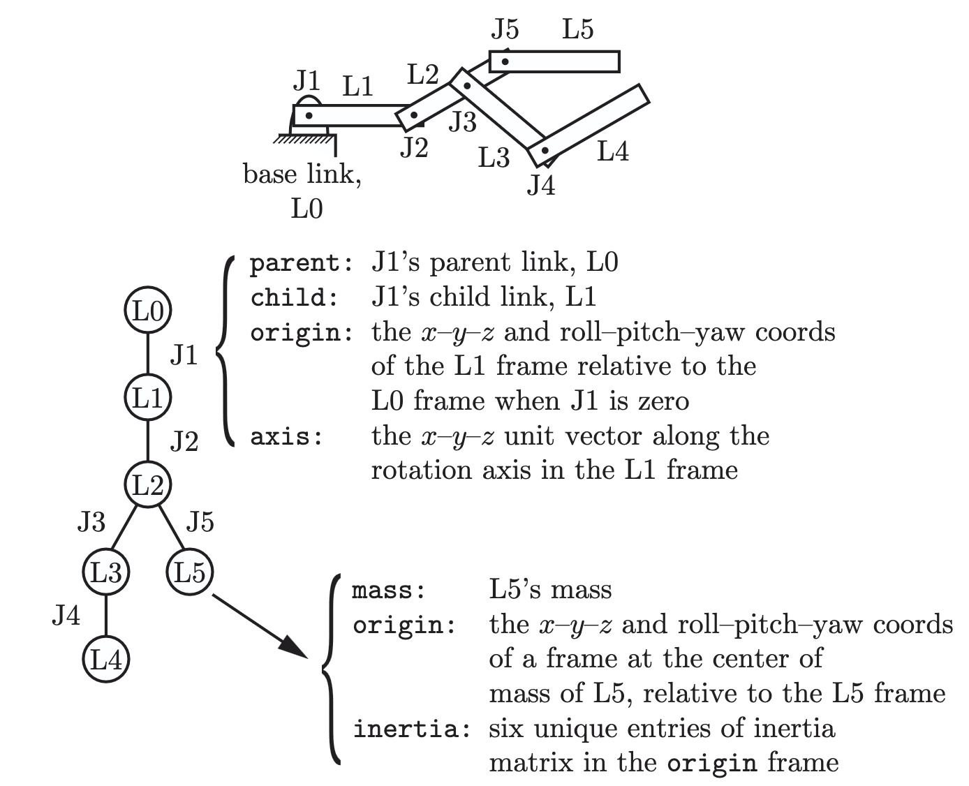
A URDF represents the robot as a tree of <link> elements connected by <joint> elements. Each joint defines exactly one <parent> and one <child> link, so the kinematic graph is necessarily acyclic.
Closed kinematic chains are therefore excluded from the model. Parallel mechanisms, four-bar linkages, and other looped topologies must be represented either in formats such as SDF or through explicit loop-closure constraints in the host simulator.
Elements
A <link> element represents a rigid body. It may contain three optional sub-elements:
-
<inertial>: the mass, center of mass, and inertia tensor, expressed in the link frame. -
<visual>: geometry used for rendering. -
<collision>: geometry used for contact detection.
Both <visual> and <collision> may specify their own <origin> relative to the link frame, allowing a single link to carry multiple visual or collision geometries.
A <joint> element specifies both the connectivity and relative motion between two links. The kinematically relevant fields are:
| Element | Description |
|---|---|
<parent link="…"> |
Parent link in the kinematic tree. |
<child link="…"> |
Child link in the kinematic tree. |
type |
Joint type (revolute, continuous, prismatic, fixed, floating, or planar). |
<origin xyz="…" rpy="…"> |
Pose of the child frame relative to the parent frame at the home configuration $q = 0$. |
<axis xyz="…"> |
Joint axis, expressed in the joint frame. |
<limit lower=… upper=… effort=… velocity=…> |
Position, effort, and velocity limits. |
<dynamics damping=… friction=…> |
Optional viscous-damping and Coulomb-friction parameters for simulation. |
The six standard joint types correspond directly to familiar rigid-body joints:
- revolute (1 DoF): rotation about a fixed axis with finite limits.
- continuous (1 DoF): rotation about a fixed axis without limits.
- prismatic (1 DoF): translation along a fixed axis.
- fixed (0 DoF): rigid attachment between two links.
- floating (6 DoF): unconstrained rigid-body motion in space.
- planar (3 DoF): motion constrained to a plane.
Among these, revolute and prismatic joints are by far the most common in manipulators and legged robots.
Frame Transformation
The kinematic contribution of a URDF joint consists of two parts: a constant origin transform $T_{\text{origin}}$ and the variable joint transform $T_{\text{joint}}(q)$.
Origin transform. The tag <origin xyz="x y z" rpy="r p y"> tag specifies the pose of the child frame relative to the parent frame at the home configuration $q = 0$. The translation is $(x,y,z)$, and the rotation is given by the fixed-axis roll–pitch–yaw convention:
Joint transform. The joint itself contributes the configuration-dependent motion. For a revolute or continuous joint with axis $\hat{\mathbf{a}}$,
\[T_{\text{joint}}(q) \;=\; \begin{bmatrix} e^{[\hat{\mathbf{a}}] q} & \mathbf{0} \\ \mathbf{0}^\top & 1 \end{bmatrix} \qquad \text{(revolute/continuous)},\]A prismatic joint contributes a translation $q\hat{\mathbf{a}}$, while a fixed joint contributes the identity. The full parent-to-child transform is
\[T_{p \to c}(q) \;=\; T_{\text{origin}}\, T_{\text{joint}}(q),\]At $q=0$, the joint transform reduces to the identity, recovering the home-pose semantics encoded by <origin>.
From URDF to PoE
The PoE formula $T(\boldsymbol{\theta}) = e^{[\mathcal{S}_1]\theta_1}\cdots e^{[\mathcal{S}_n]\theta_n}\, M$ can be extracted directly from a URDF in two passes along the kinematic chain.
Pass 1: Home configuration $M$. Setting all joint variables to zero removes the joint transforms, leaving only the origin transforms. Chaining them gives the home pose
\[M \;=\; T_{\text{origin}}^{(1)}\, T_{\text{origin}}^{(2)}\, \cdots\, T_{\text{origin}}^{(n)},\]This is the end-effector pose relative to the base when all joint coordinates are zero.
Pass 2: Screw Axes $\mathcal{S}_i$. Each URDF joint stores an axis \(\hat{\mathbf{a}}_i\) in its local frame. Expressing the same axis in the base frame requires propagating it through the corresponding home transforms. Let
\[R_{0 \to i}^{\text{home}} \;=\; \text{rotation part of } T_{\text{origin}}^{(1)} \cdots T_{\text{origin}}^{(i)}, \qquad \mathbf{q}_i \;=\; \text{translation part of the same product},\]so $\mathbf{q}_i$ is a point on the joint-$i$ axis at the home pose. For a revolute joint,
\[\hat{\boldsymbol{\omega}}_i \;=\; R_{0 \to i}^{\text{home}}\, \hat{\mathbf{a}}_i, \qquad \mathbf{v}_i \;=\; -\hat{\boldsymbol{\omega}}_i \times \mathbf{q}_i,\]giving the spatial screw axis \(\mathcal{S}_i = (\hat{\boldsymbol{\omega}}_i,\, \mathbf{v}_i)\). For a prismatic joint,
\[\mathcal{S}_i = (\mathbf{0},\, R_{0 \to i}^{\text{home}}\, \hat{\mathbf{a}}_i).\]The resulting set \((M,\, \mathcal{S}_1, \ldots, \mathcal{S}_n)\) is precisely the PoE description of the robot.
This is precisely what libraries such as pinocchio::buildModel, and drake::multibody::Parser, do internally: parse the URDF, traverse the kinematic tree, and construct the home configuration, screw axes, and inertial parameters required for dynamics algorithms.
Limitations and Adjacent Formats
URDF was designed for single-robot, tree-structured, rigid-body systems. As a consequence, the most consequential limitations are:
- No closed kinematic chains. Parallel mechanisms (Stewart platforms, five-bar linkages) and loop-closing constraints must be added on top, typically via the simulator's bilateral-constraint API.
- No multi-robot scenes or environments. Tables, walls, sensors not rigidly attached to the robot, and other robots live outside the URDF; they are described in companion files (`world`, `xacro`, SDF scenes).
- No semantic layer. Concepts such as end-effectors, gripper groups, mimicked joints (one joint that copies another's value), and self-collision exclusions are not part of the URDF schema; they are usually carried in a parallel SRDF (Semantic Robot Description Format) file consumed by motion planners.
These limitations are addressed by related formats. SDF (Simulation Description Format), originally from Gazebo, extends the model to complete simulation worlds and supports richer physics annotations. MJCF, MuJoCo’s native XML, supports closed chains, soft constraints, and contact-rich behaviour with finer control over contact parameters. Xacro is a macro layer on top of URDF that expands at build time, allowing parameterized robot descriptions to be shared across variants of the same mechanism.
Despite these limitations, URDF remains the standard robot-description format for manipulators and legged robots. Its tree structure maps directly onto the Product-of-Exponentials formulation developed in this chapter.
Summary
The forward kinematics map $\boldsymbol{\theta} \mapsto T(\boldsymbol{\theta}) \in SE(3)$ admits two dominant parameterizations. Denavit–Hartenberg (DH) parameters describe a manipulator through a sequence of local coordinate frames, whereas the Product-of-Exponentials (PoE) formulation describes it through screw axes and the exponential map. Side by side:
| Aspect | DH Parameters | Product of Exponentials |
|---|---|---|
| Origin | Denavit & Hartenberg (1955) | Brockett (1984) |
| Parameters per joint | 4 ($a_i, \alpha_i, d_i, \theta_i$) | 6 (screw axis $\mathcal{S}_i$) |
| Number of frames | $n + 1$ (one per link) | 2 (base \(\{s\}\) and body \(\{b\}\)) |
| Per-joint transform | $A_i = \mathrm{Rot}_z\,\mathrm{Trans}_z\,\mathrm{Trans}_x\,\mathrm{Rot}_x$ | $e^{[\mathcal{S}_i]\theta_i}$ |
| End-effector pose | $T = A_1 A_2 \cdots A_n$ | $T = e^{[\mathcal{S}_1]\theta_1} \cdots e^{[\mathcal{S}_n]\theta_n}\, M$ |
| Revolute/prismatic handling | Separate conventions | Unified formulation |
| Geometric transparency | Indirect (encoded in 4-tuple per link) | Direct (screw axis is the joint axis) |
| Parallel-axis singularity | Yes (common normal ill-defined) | No (formula is uniform) |
| Velocity kinematics | Requires extra derivation | Jacobian follows naturally |
Both formulations produce the same $T(\boldsymbol{\theta})$ for the same robot; for the planar 3R arm both reduce to the familiar end-effector position
\[\mathbf{p}(\boldsymbol{\theta}) = \bigl(L_1 \cos\theta_1 + L_2 \cos(\theta_1+\theta_2) + L_3 \cos(\theta_1+\theta_2+\theta_3),\; L_1 \sin\theta_1 + L_2 \sin(\theta_1+\theta_2) + L_3 \sin(\theta_1+\theta_2+\theta_3),\; 0\bigr).\]n modern robotics software, PoE aligns naturally with URDF-based robot models and extends cleanly to Jacobians, dynamics, and control. DH remains useful for compact analytic derivations and closed-form inverse kinematics, but PoE has become the dominant representation in contemporary robotics libraries.
The remainder of this series adopts the PoE formulation. The next post differentiates the PoE chain to derive the spatial and body Jacobians, $J_s$ and $J_b$, and uses them to characterize kinematic singularities.
Reference
[1] John J. Craig, Introduction to Robotics: Mechanics and Control, 3rd Edition, Pearson Prentice Hall, 2005. Chapter 3.
[2] Mark W. Spong, Seth Hutchinson, and M. Vidyasagar, Robot Dynamics and Control, 2nd Edition, January 2004. Chapter 3.
[3] Kevin M. Lynch and Frank C. Park, Modern Robotics: Mechanics, Planning, and Control, Cambridge University Press, 2017. Chapter 4 and Appendix C.
[4] J. Denavit and R. S. Hartenberg, “A kinematic notation for lower-pair mechanisms based on matrices,” ASME Journal of Applied Mechanics, 22:215-221, 1955.
[5] R. W. Brockett, “Robotic manipulators and the product of exponentials formula,” in Mathematical Theory of Networks and Systems, pp. 120-129, Springer, 1984.
Leave a comment